7 Additional material: exact solutions and basis functions

From fitting a line to learning a representation

Optional route after the main chapter

Depth choice: the closed-form derivation extends W01-02 and W01-03. Enrichment: basis functions extend the model discussion in W01-01 and prepare for feed-forward neural networks. These sections do not add prerequisites to the common-core path or change its assessment requirements.

Allow about 45–60 minutes for the worked material, plus time for an exercise. This notebook runs independently from a fresh kernel. It assumes the main chapter’s partial derivatives and gradient notation; maximum likelihood is not required.

We ask two separate questions: Can we find the best line directly? And what if even the best line has the wrong shape? The second question follows the same try → understand → improve cycle as the main chapter.

7.1 One parameter, coordinate solves, and the joint solve

The first model in the main chapter is \(\hat y=wx\), with bias fixed at zero. Its objective and derivative are

\[ L_0(w)=\frac1n\sum_i(y^{(i)}-wx^{(i)})^2, \qquad \frac{dL_0}{dw}=-\frac2n\sum_i(y^{(i)}-wx^{(i)})x^{(i)}. \]

When \(\sum_i(x^{(i)})^2>0\), setting this derivative to zero gives

\[ w_0^*=\frac{\sum_i x^{(i)}y^{(i)}}{\sum_i(x^{(i)})^2}. \]

This is an exact optimum within the origin-passing model family. It does not repair a missing offset. If every input is zero, predictions do not depend on the weight and it cannot be identified from those data.

After introducing a bias, solving for weight at fixed bias \(b_t\) replaces each target by \(y^{(i)}-b_t\):

\[ w_{t+1}=\frac{\sum_i x^{(i)}(y^{(i)}-b_t)}{\sum_i(x^{(i)})^2}, \qquad b_{t+1}=\bar y-w_{t+1}\bar x. \]

Alternating these exact one-variable minima is coordinate descent. Each step cannot increase the full squared-error objective, but the other coordinate changes the location of its next minimum. The formulas below instead solve both stationary equations together. Distinguish that joint solution from alternating coordinate solves and from taking small gradient steps.

7.2 Find the best line without taking small steps

The main chapter compared coordinate descent, single-example SGD, batch descent, and torch.linalg.lstsq. The direct solve served as an independent reference. Here we derive what the solver computes. A closed-form solution expresses the fitted parameters directly in terms of the data, instead of defining them through repeated gradient updates.

For \(n\) observations, the model and objective are

\[ \hat y^{(i)}=wx^{(i)}+b,\qquad L(w,b)=\frac1n\sum_{i=1}^n(y^{(i)}-(wx^{(i)}+b))^2. \]

The measured \(x^{(i)},y^{(i)}\) are fixed. Only \(w,b\) are unknown. Multiplying the objective by \(n\) would not change its minimizer.

7.2.1 Step 1: solve the bias equation

At a minimum, the two partial derivatives are zero. Start with the bias:

\[ 0=\frac{\partial L}{\partial b} =-\frac2n\sum_i(y^{(i)}-(wx^{(i)}+b)). \]

Define the sample means \(\bar x=n^{-1}\sum_i x^{(i)}\) and \(\bar y=n^{-1}\sum_i y^{(i)}\). Dividing the equation by 2 gives

\[ w\bar x+b-\bar y=0 \quad\Longrightarrow\quad \boxed{b=\bar y-w\bar x}. \]

Thus every stationary fit with a bias passes through \((\bar x,\bar y)\). Once the weight is known, the bias is determined.

7.2.2 Step 2: substitute into the weight equation

With that bias, each residual becomes

\[ r^{(i)}=(y^{(i)}-\bar y)-w(x^{(i)}-\bar x). \]

The weight equation from the main chapter is \(\sum_i x^{(i)}r^{(i)}=0\). The bias equation also gives \(\sum_i r^{(i)}=0\), so subtracting \(\bar x\sum_i r^{(i)}\) changes nothing. Therefore

\[ \begin{aligned} 0 &=\sum_i(x^{(i)}-\bar x)r^{(i)}\\ &=\sum_i(x^{(i)}-\bar x)(y^{(i)}-\bar y) -w\sum_i(x^{(i)}-\bar x)^2. \end{aligned} \]

If the inputs are not all equal, the denominator below is positive and we obtain

\[ \boxed{ w^*=\frac{\sum_i(x^{(i)}-\bar x)(y^{(i)}-\bar y)} {\sum_i(x^{(i)}-\bar x)^2}, \qquad b^*=\bar y-w^*\bar x. } \]

The numerator measures how centered inputs and targets vary together; the denominator measures the input variation. If you know sample covariance and variance from Math 3, this is their ratio when both use the same normalization. That statistical vocabulary is not needed for the derivation.

7.2.3 Step 3: check the condition and the result

If all inputs equal a constant \(c\), the denominator is zero. The best constant prediction is still \(\bar y\), but any parameters satisfying \(wc+b=\bar y\) produce it. The data cannot identify the slope separately from the bias. This is a lack of information, not a reason to divide by a tiny arbitrary number.

The following noisy example compares the derived formula with an independent least-squares solver. It also checks that the mean fitted residual is zero.

import matplotlib.pyplot as plt
from dlbook.plotting import show_plot
import torch

DTYPE = torch.float64
rng_line = torch.Generator().manual_seed(31)
x_line = torch.linspace(-2, 2, 30, dtype=DTYPE)
y_line = 1.6 * x_line + 0.45 + 0.2 * torch.randn(30, generator=rng_line, dtype=DTYPE)
x_mean, y_mean = x_line.mean(), y_line.mean()
x_centered, y_centered = x_line - x_mean, y_line - y_mean
input_variation = x_centered.square().sum()
assert input_variation > 0
w_closed = (x_centered * y_centered).sum() / input_variation
b_closed = y_mean - w_closed * x_mean

# One column per parameter, in the order [weight, bias].
A_line = torch.stack((x_line, torch.ones_like(x_line)), dim=1)
solver_parameters = torch.linalg.lstsq(A_line, y_line[:, None]).solution[:, 0]
torch.testing.assert_close(torch.stack((w_closed, b_closed)), solver_parameters)
residual_line = y_line - (w_closed * x_line + b_closed)
torch.testing.assert_close(residual_line.mean(), torch.tensor(0.0, dtype=DTYPE),
                           atol=1e-12, rtol=0)
print(f"Closed-form weight={w_closed.item():.4f}, bias={b_closed.item():.4f}")

Closed-form weight=1.5829, bias=0.5399

The next derivation explains why a stationary solution is a global minimum, rather than merely asserting that setting derivatives to zero always suffices.

7.3 The same derivation for several features

Let \(\mathbf X\) be the \(n\times d\) matrix with examples in rows and features in columns. Add a column of ones for the bias:

\[ \mathbf A=[\mathbf X\;\mathbf 1]\in\mathbb R^{n\times p}, \qquad \boldsymbol\theta=\begin{bmatrix}\mathbf w\\b\end{bmatrix}\in\mathbb R^p, \qquad p=d+1. \]

There are \(p\) parameters in total. The target column is \(\mathbf y\in\mathbb R^n\), and the prediction column is \(\mathbf A\boldsymbol\theta\). The objective is

\[ L(\boldsymbol\theta)=\frac1n\|\mathbf y-\mathbf A\boldsymbol\theta\|_2^2. \]

The squared norm means the sum of squared entries. We can derive the matrix expression using only individual partial derivatives. For entry \(\theta_j\),

\[ \frac{\partial L}{\partial\theta_j} =-\frac2n\sum_i A_{ij}\left(y^{(i)}-\sum_k A_{ik}\theta_k\right). \]

Collecting these entries gives

\[ \nabla L=-\frac2n\mathbf A^\top(\mathbf y-\mathbf A\boldsymbol\theta). \]

Setting the gradient to zero produces the normal equations:

\[ \boxed{\mathbf A^\top\mathbf A\boldsymbol\theta^*=\mathbf A^\top\mathbf y}. \]

If the columns of \(\mathbf A\) are linearly independent (full column rank), then \(\mathbf A^\top\mathbf A\) is invertible and the unique solution is

\[ \boxed{\boldsymbol\theta^*=(\mathbf A^\top\mathbf A)^{-1}\mathbf A^\top\mathbf y}. \]

Full column rank requires at least as many observations as parameters, but \(n\geq p\) alone does not guarantee it: duplicate or redundant feature columns still prevent identification.

7.3.1 Why this is a global minimum

Let \(\mathbf r^*=\mathbf y-\mathbf A\boldsymbol\theta^*\). The normal equations state \(\mathbf A^\top\mathbf r^*=0\): the residual is orthogonal to every design column. For any parameter change \(\boldsymbol\delta\),

\[ \begin{aligned} L(\boldsymbol\theta^*+\boldsymbol\delta) &=\frac1n\|\mathbf r^*-\mathbf A\boldsymbol\delta\|_2^2\\ &=L(\boldsymbol\theta^*) -\frac2n\boldsymbol\delta^\top\mathbf A^\top\mathbf r^* +\frac1n\|\mathbf A\boldsymbol\delta\|_2^2\\ &=L(\boldsymbol\theta^*)+\frac1n\|\mathbf A\boldsymbol\delta\|_2^2 \geq L(\boldsymbol\theta^*). \end{aligned} \]

No change can reduce the objective further. With full column rank, a nonzero change cannot satisfy \(\mathbf A\boldsymbol\delta=0\), so the minimum is unique. Without full rank, multiple parameter vectors can give the same fitted training predictions. The pseudoinverse expression \(\boldsymbol\theta^*=\mathbf A^+\mathbf y\) selects a minimum-norm least-squares solution; deriving the pseudoinverse is beyond this chapter.

7.3.2 A formula is not necessarily the best numerical algorithm

The inverse expression explains the optimum. In software, use torch.linalg.lstsq(A, y) rather than explicitly forming the inverse. Forming \(\mathbf A^\top\mathbf A\) can amplify numerical problems when columns are nearly dependent. Least-squares solvers can work directly with the design matrix using suitable factorizations. For these small, well-conditioned, full-rank examples, the default CPU solver is sufficient.

We can check both the normal equations and the global-minimum identity on the earlier data:

theta = solver_parameters[:, None]
target_column = y_line[:, None]
r_star = target_column - A_line @ theta
torch.testing.assert_close(A_line.T @ r_star, torch.zeros((2, 1), dtype=DTYPE),
                           atol=1e-10, rtol=0)
delta = torch.tensor([[0.3], [-0.2]], dtype=DTYPE)
loss_at_solution = r_star.square().mean()
loss_after_change = (A_line @ (theta + delta) - target_column).square().mean()
extra_loss = (A_line @ delta).square().mean()
torch.testing.assert_close(loss_after_change, loss_at_solution + extra_loss)
print(f"MSE at solution: {loss_at_solution.item():.4f}")
print(f"MSE after changing parameters: {loss_after_change.item():.4f}")

MSE at solution: 0.0310
MSE after changing parameters: 0.1993

These arguments require no Gaussian noise assumption. Gaussian maximum likelihood supplies an additional interpretation under the assumptions stated in the main chapter.

7.4 Try: even the best line can fail

Now use a new synthetic calibration process with a curved relationship. The generating formula is visible so the example is reproducible; the fitting procedures use only their training rows. Split once into 54 training, 18 validation, and 18 test examples. We keep the test targets out of model selection.

Predict before running: if a straight line leaves a systematic pattern in its residuals, will more gradient-descent steps necessarily remove that pattern?

rng_curve = torch.Generator().manual_seed(37)
x_all = torch.linspace(-2, 2, 90, dtype=DTYPE)
y_all = 0.4 + 0.8 * x_all + 0.9 * x_all.square()
y_all = y_all + 0.2 * torch.randn(90, generator=rng_curve, dtype=DTYPE)
permutation = torch.randperm(90, generator=rng_curve)
train, valid, test = permutation[:54], permutation[54:72], permutation[72:]
x_train, y_train = x_all[train], y_all[train, None]
x_valid, y_valid = x_all[valid], y_all[valid, None]
x_test, y_test = x_all[test], y_all[test, None]

# This is the exact least-squares fit within the straight-line model family.
A_train = torch.stack((torch.ones_like(x_train), x_train), dim=1)
coef_affine = torch.linalg.lstsq(A_train, y_train).solution
pred_affine = A_train @ coef_affine
assert pred_affine.shape == y_train.shape == (54, 1)
grid = torch.linspace(-2, 2, 201, dtype=DTYPE)
affine_grid = coef_affine[0, 0] + coef_affine[1, 0] * grid

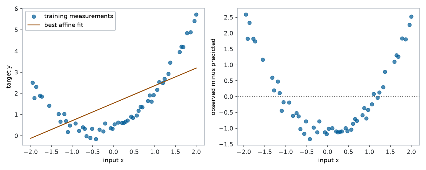
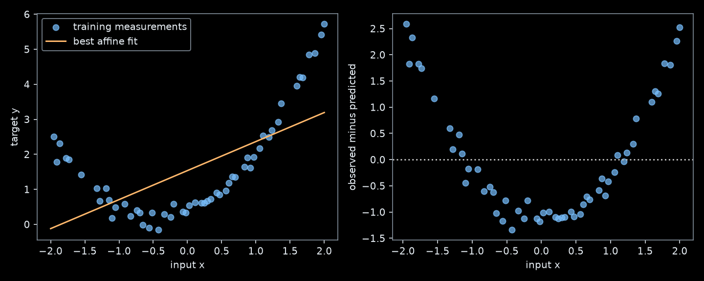
Two panels show curved synthetic training data with a straight-line fit, and residuals forming a U-shaped pattern against the input. — Figure 7.1: An optimally fitted straight line leaves curved structure in the training residuals. The issue is the model family, not an unfinished optimizer.

With residuals defined as observed minus predicted, the upward-curved targets leave a U-shaped residual pattern. The line is already the least-squares optimum in its family. Improving the optimizer cannot make that family contain a quadratic curve.

7.5 Understand: linear in which quantities?

Instead of feeding the original input directly to the model, first compute a set of fixed feature functions, often called basis functions:

\[ \phi_0(x)=1,\qquad\phi_1(x)=x,\qquad\phi_2(x)=x^2. \]

Fit their weighted sum:

\[ \hat y=\theta_0\phi_0(x)+\theta_1\phi_1(x)+\theta_2\phi_2(x) =\theta_0+\theta_1x+\theta_2x^2. \]

This can be nonlinear in the original input \(x\) while remaining linear in the fitted coefficients \(\boldsymbol\theta\). The square is computed before those coefficients act. Therefore we can still fit them by linear least squares.

The word “basis” here describes a feature construction; it does not guarantee that the functions or their sampled columns are linearly independent. Rank must still be checked for a unique coefficient solution.

For \(m\) fixed functions, define the design matrix

\[ \boldsymbol\Phi_{ij}=\phi_j(x^{(i)}),\qquad \hat{\mathbf y}=\boldsymbol\Phi\boldsymbol\theta. \]

There is one row per example and one column per function. The constant function already supplies the bias; do not add a second bias column. With full column rank, the same derivation gives

\[ \boldsymbol\theta^*=(\boldsymbol\Phi^\top\boldsymbol\Phi)^{-1} \boldsymbol\Phi^\top\mathbf y. \]

Only the representation of the input changed. The squared-error objective and least-squares fitting method remain the same.

7.6 Improve: fit the curve with fixed polynomial features

Controlled hypothesis: adding the pre-specified feature \(x^2\) can reduce the systematic residual pattern on these data. Keep the split, targets, MSE objective, and direct solver fixed; change the feature map from \((1,x)\) to \((1,x,x^2)\). Model capacity changes with that map, so this is not a comparison at a fixed parameter count.

def polynomial_features(values, degree):
    # Shape (n,) -> (n, degree + 1). The first column is the bias feature.
    return torch.stack([values**power for power in range(degree + 1)], dim=1)


Phi_train = polynomial_features(x_train, degree=2)
Phi_valid = polynomial_features(x_valid, degree=2)
Phi_grid = polynomial_features(grid, degree=2)
assert Phi_train.shape == (54, 3)
assert torch.linalg.matrix_rank(Phi_train).item() == 3
coef_quadratic = torch.linalg.lstsq(Phi_train, y_train).solution
pred_quadratic = Phi_train @ coef_quadratic
mse_affine = (pred_affine - y_train).square().mean()
mse_quadratic = (pred_quadratic - y_train).square().mean()
assert mse_quadratic < mse_affine
print("Quadratic coefficients [constant, x, x squared]:", coef_quadratic[:, 0].tolist())
print(f"Training MSE: affine={mse_affine.item():.4f}; quadratic={mse_quadratic.item():.4f}")

Quadratic coefficients [constant, x, x squared]: [0.3592121211518583, 0.7934467029103465, 0.9238453011218243]
Training MSE: affine=1.3317; quadratic=0.0278

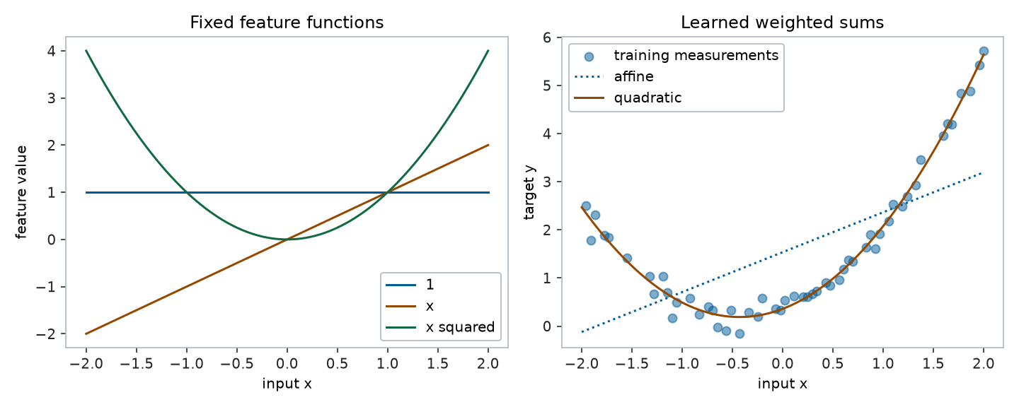
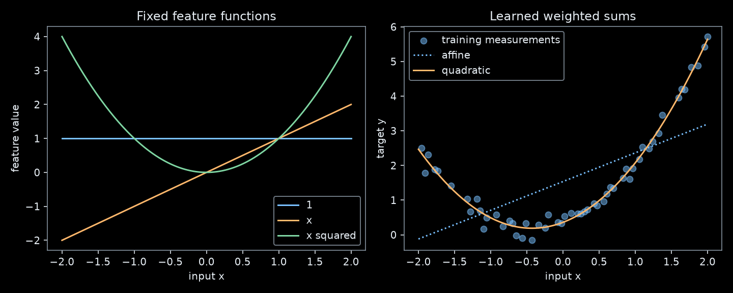
The left panel shows the constant, identity, and square feature functions. The right panel compares affine and quadratic fitted curves against the same synthetic training measurements. — Figure 7.2: Fixed polynomial features are combined with learned coefficients. The quadratic fit follows the curved training relationship while using the same least-squares solver.

Because the affine model is contained in the quadratic model by setting \(\theta_2=0\), the exact minimum training MSE cannot increase when this feature is added. That nesting argument says nothing about held-out performance: extra features can also fit noise. High polynomial degrees can create unstable extrapolation and nearly dependent columns. Choose feature maps using training/validation data, and preserve the test set for the final check.

7.7 Another feature family: fixed ReLU hinges

Polynomial powers are not the only choice. A rectified linear unit, abbreviated ReLU, is the function

\[ \operatorname{ReLU}(z)=\max(0,z). \]

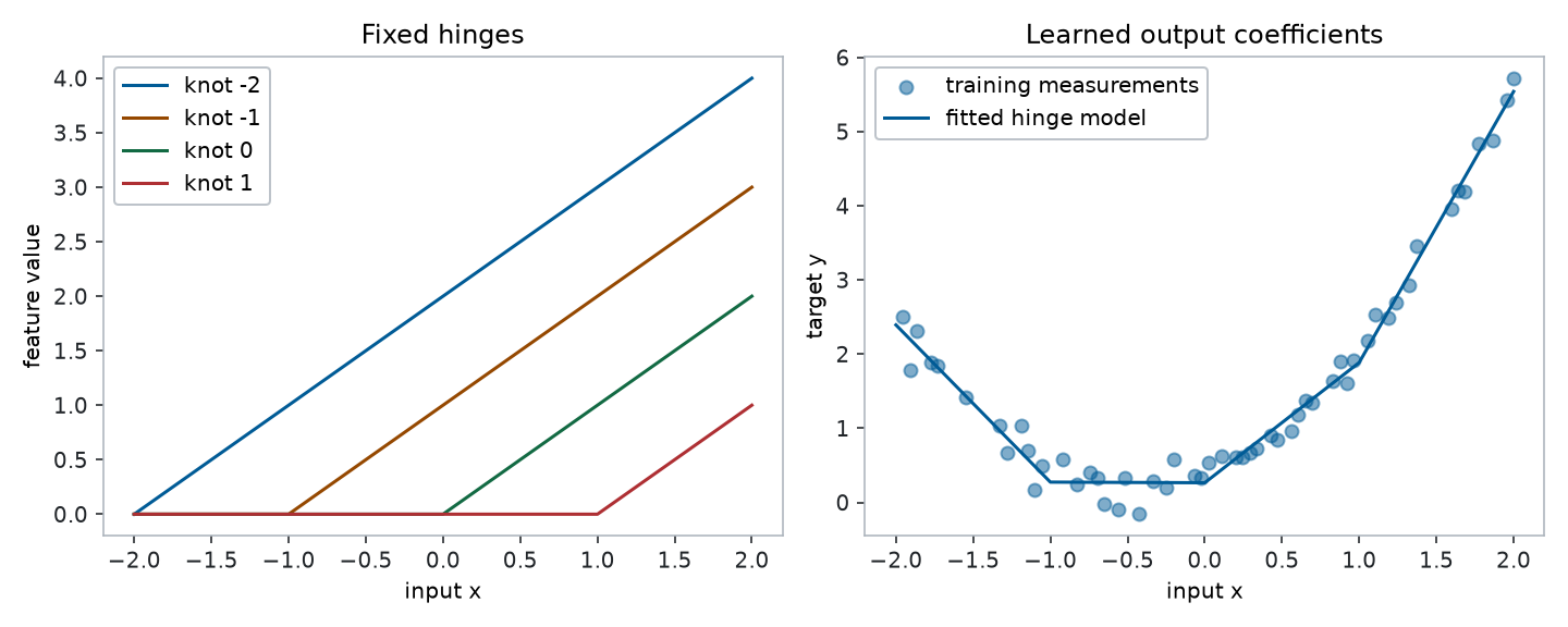
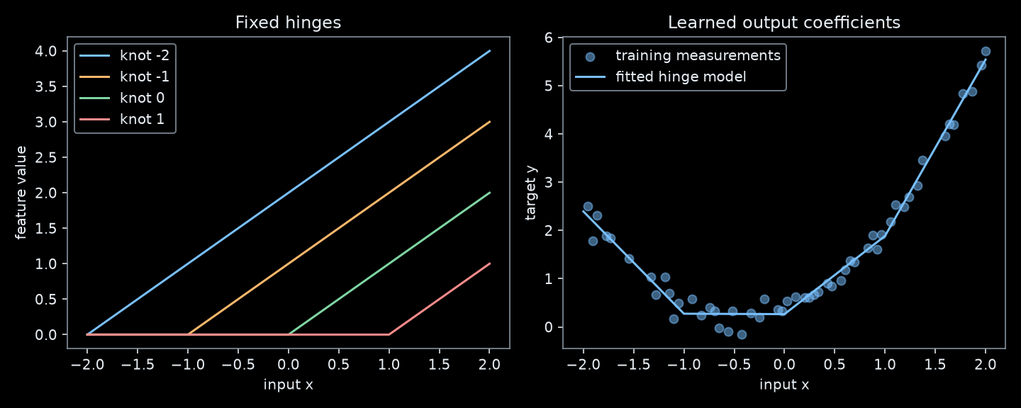
For a fixed location \(t_j\), the function \(\phi_j(x)=\operatorname{ReLU}(x-t_j)\) is zero to the left of \(t_j\) and rises linearly to the right. The location is called a knot here. A weighted sum of these hinges produces a continuous, piecewise-linear curve: each coefficient changes its slope at a knot.

For this experiment, fix four knots in advance at \(-2,-1,0,1\), covering the declared input range. Fit only a constant and the four output coefficients. This remains linear least squares, even though the feature functions are nonlinear in \(x\).

knots = torch.tensor([-2.0, -1.0, 0.0, 1.0], dtype=DTYPE)


def hinge_features(values):
    hinges = torch.relu(values[:, None] - knots[None, :])  # (n, 4)
    return torch.cat((torch.ones((len(values), 1), dtype=values.dtype), hinges), dim=1)


H_train, H_valid, H_grid = [hinge_features(v) for v in (x_train, x_valid, grid)]
assert H_train.shape == (54, 5)
assert torch.linalg.matrix_rank(H_train).item() == 5
coef_hinges = torch.linalg.lstsq(H_train, y_train).solution
# Verify that explicit weighted addition is the same prediction rule.
explicit_prediction = coef_hinges[0, 0] + (
    H_grid[:, 1:] * coef_hinges[1:, 0]
).sum(dim=1)
torch.testing.assert_close(explicit_prediction, (H_grid @ coef_hinges)[:, 0])

The left panel shows four zero-then-rising ReLU features with different fixed knots. The right panel shows their learned piecewise-linear combination following the curved data. — Figure 7.3: Fixed ReLU hinges and their fitted weighted sum. A neural network will also learn the transformations that determine its features.

Compare the three pre-specified feature maps on validation data, then freeze the choice. Their parameter counts are 2, 3, and 5 respectively; this example demonstrates representations, not a general ranking of model families.

candidates = {
    "affine": (lambda v: polynomial_features(v, 1), coef_affine),
    "quadratic": (lambda v: polynomial_features(v, 2), coef_quadratic),
    "fixed hinges": (hinge_features, coef_hinges),
}
validation_mse = {}
for name, (feature_map, coefficients) in candidates.items():
    validation_mse[name] = (feature_map(x_valid) @ coefficients - y_valid).square().mean().item()
    print(f"{name:14s} validation MSE={validation_mse[name]:.4f}")
selected = min(validation_mse, key=validation_mse.get)
print("Choice frozen before test evaluation:", selected)

affine         validation MSE=1.0993
quadratic      validation MSE=0.0376
fixed hinges   validation MSE=0.0504
Choice frozen before test evaluation: quadratic

The next cell uses test targets only to evaluate that frozen choice. If you keep changing features after seeing its score, this split is no longer an untouched test set.

chosen_map, chosen_coefficients = candidates[selected]
test_prediction = chosen_map(x_test) @ chosen_coefficients
assert test_prediction.shape == y_test.shape
test_rmse = (test_prediction - y_test).square().mean().sqrt().item()
print(f"Final held-out RMSE for {selected}: {test_rmse:.4f}")

Final held-out RMSE for quadratic: 0.1986

These small synthetic data establish an executable example, not an advantage of one family on arbitrary problems or outside the sampled input range.

7.8 From fixed basis functions to neural networks

So far, we designed every feature function. Why should our choice of powers or hinge locations suit every prediction problem? A neural network makes the feature construction itself trainable.

For one scalar input, a one-hidden-layer regression network can be written as

\[ \phi_j(x;a_j,c_j)=\operatorname{ReLU}(a_jx+c_j),\qquad \hat y=\beta_0+\sum_{j=1}^m\beta_j\phi_j(x;a_j,c_j). \]

Here \(a_j,c_j\) determine hidden feature \(j\); \(\beta_j\) is its output weight and \(\beta_0\) is the output bias. Our fixed-hinge model is the special case \(a_j=1,c_j=-t_j\), with only the \(\beta\) parameters fitted. Learning the hidden parameters changes the locations, orientations, and scales of the feature responses. It does not guarantee a better held-out fit.

The following forward calculation verifies this correspondence without introducing a new training algorithm:

hidden_weights = torch.ones_like(knots)
hidden_biases = -knots
hidden_activations = torch.relu(
    grid[:, None] * hidden_weights[None, :] + hidden_biases[None, :]
)
network_output = hidden_activations @ coef_hinges[1:] + coef_hinges[0]
torch.testing.assert_close(network_output, H_grid @ coef_hinges)
print("Fixed-basis prediction equals a network with frozen hidden parameters.")

Fixed-basis prediction equals a network with frozen hidden parameters.

If the hidden parameters are held fixed, fitting the final linear layer with MSE is still a least-squares problem. If they are learned jointly, the feature matrix depends on unknown parameters. There is no single application of the fixed-design normal-equation formula that solves that joint problem. Gradient-based training and the chain rule become useful again; their network implementation is the topic of Week 4.

A deep network composes several such feature transformations. Let \(\mathbf h^{(0)}=\mathbf x\) denote the original feature vector. At layer \(\ell\), form

\[ \mathbf h^{(\ell)}=\sigma\!\left(\mathbf W^{(\ell)}\mathbf h^{(\ell-1)}+\mathbf c^{(\ell)}\right), \qquad \hat y=\boldsymbol\beta^\top\mathbf h^{(L)}+\beta_0. \]

The matrix \(\mathbf W^{(\ell)}\) and bias \(\mathbf c^{(\ell)}\) are learned; \(\sigma\) applies a nonlinear activation such as ReLU to each entry. Each layer can combine features produced by the previous one. If all activations were the identity, composing the affine layers would give another affine map, so depth alone would not produce a nonlinear input-output relationship.

Model	Feature construction	Parameters fitted in this example
Ordinary affine regression	Original input and a constant	Slope and bias
Polynomial regression	Fixed powers of the input	Output coefficients
Fixed-hinge regression	ReLU features with chosen knots	Output coefficients
One-hidden-layer network	Parameterized feature responses	Hidden parameters and output coefficients
Deep network	Several composed feature transformations	Parameters throughout the layers

The connection to DNNs is therefore a concrete extension of something already understood: a linear readout of features, with increasingly flexible ways to construct and learn those features.

7.9 Exercises — optional

7.9.1 Mathematics bridge

Depth choice: derive \(w^*,b^*\) for \(x=(0,1,2)\) and \(y=(1,2,2)\) using centered sums. Verify that the residuals sum to zero. Which step fails when \(x=(1,1,1)\)?
Depth choice: explain every term in the global-minimum identity. Why does a zero gradient alone not prove a global minimum for an arbitrary nonlinear objective?

7.9.2 Coding bridge

Depth choice: construct the three polynomial columns for five chosen inputs without a loop. Verify the result against polynomial_features and state both dimensions.
Depth choice: add a duplicate constant column to a design matrix. Inspect its rank and explain why coefficients need not be unique, even when fitted predictions are.

7.9.3 Stretch

Enrichment: change the feature map to include \(x^3\) as well. Before fitting, predict what must happen to the optimum training MSE and what need not happen to validation MSE. Keep the split fixed and leave test targets unopened until your final choice.
Enrichment: move one fixed ReLU knot and refit the output coefficients. Describe which part of the model you changed. Contrast this manual design choice with learning the hidden parameters jointly.
Enrichment: algebraically collapse two affine layers with identity activations into one. Explain why the nonlinear activation matters to the basis-function motivation.

7.10 Summary

Closed-form least squares identifies the best fit within a chosen linear-in-parameters model. It cannot repair a model family with the wrong shape. Fixed basis functions expand that family while preserving the linear least-squares fitting problem. Learning the feature construction, and composing it across layers, provides the next step toward neural networks.

Return to the main chapter or the lab. Continue the learned-feature idea in Week 4.