5 Week 1: Linear Regression

From a supervised problem to a fitted line

Your route through the chapter

Predict → try → explain → fit. First identify a supervised learning problem and try a one-parameter model. Then add a bias, define squared error, and turn familiar partial derivatives into fitting procedures. We introduce single-example stochastic updates before averaging derivatives over a batch, and finish with a direct least-squares solve.

When	What you do
Before Session 1	Nothing: no preparation or installation is assumed.
Session 1, 90 minutes	Course introduction and survey; supervised regression; setup and hand trials; derivatives; coordinate descent; gradient; SGD; batch descent; direct solve.
Between sessions	Optional consolidation only.
Session 2, 90 minutes	Reconstruct the updates, diagnose training failures, and begin the lab.
After Session 2	Finish the lab and explain the evidence; allow about 3–4 hours.

Run Python cells from top to bottom. The examples use PyTorch and Matplotlib on CPU, with no data downloads. A rendered page displays results; editing a cell requires a notebook or Quarto editor. The in-class exercise setup and worksheet provide the short runnable route through Monday’s discussion.

5.1 Starting points and learning outcomes

We recall partial derivatives, including the chain rule, before introducing the gradient vector. No probability or Math 3 course is required for the common route. Basic Python support is provided independently of mathematics support: being comfortable with one does not imply being comfortable with the other.

If you took Math 3, you may recognize least squares and maximum likelihood. Use that familiarity to check your reasoning, but still work through the shared experiment. The statistical connections occur after that experiment.

W01-01 — Common core: identify input, target, and parameters in supervised regression; formulate one-parameter and affine predictors and MSE.
W01-02 — Common core: build a gradient from partial derivatives, check it numerically, and explain a local update.
W01-03 — Common core: compare exact coordinate descent, single-example SGD, full-batch descent, and direct least squares.
W01-04 — Common core: diagnose learning-rate and feature-scale failures; separate fitting from held-out evaluation.

Depth choice: least-squares derivation and Gaussian maximum likelihood. Enrichment: conditioning and extrapolation investigations in the lab. Neither assumes that all students took Math 3.

5.2 First: what is a supervised learning problem?

A sensor produces a reading \(x\). A reference instrument supplies the quantity \(y\) that we want to predict. During training we have paired examples: for each input, we also know a target answer. That pairing makes this a supervised learning problem. At prediction time, a new sensor reading is available, but its reference target is not.

For example \(i\), write the observed input as \(x^{(i)}\) and the observed target as \(y^{(i)}\). The superscript \(i\) labels an example; it is not a power. A model is a prediction rule with adjustable parameters \(\boldsymbol\theta\):

\[ \hat y^{(i)}=f_{\boldsymbol\theta}(x^{(i)}). \tag{5.1}\]

A hat distinguishes a prediction from an observed target. Learning chooses parameters using the training pairs; it does not change those measurements. We need a rule for making predictions, a way to score their errors, and a procedure for changing parameters. Those are three separate choices.

Quantity	Sensor example	Available when predicting a new example?
Input \(x\)	Sensor reading	Yes
Target \(y\)	Reference measurement	Usually no
Prediction \(\hat y\)	Model’s estimate of the reference	Computed from the input
Parameters \(\boldsymbol\theta\)	Numbers chosen during fitting	Stored after training

The ultimate goal is useful predictions on new examples, not merely agreement with answers already seen. Our finite training score is an empirical score: it averages errors on the recorded examples. The corresponding population goal concerns errors on future examples from the intended measurement process. We cannot inspect all future examples, so we reserve some measured pairs for checking generalization later. This distinction needs no probability notation; a precise expected-loss definition comes after the common experiment.

5.2.1 Regression predicts a numerical quantity

Regression predicts a numerical target, such as a temperature, a price, or a reference measurement. Classification predicts a category, such as “faulty” or “working.” The input can be a number, a vector, an image, or something else; the kind of target determines this distinction. A numerical code for a category does not make it a regression target.

Quick check: predicting tomorrow’s temperature is regression; predicting whether it will rain is classification. Our sensor-calibration target is a numerical quantity, so we start with regression.

5.3 Try: can you calibrate a sensor?

The measurements below are synthetic, in arbitrary units: a teaching example, not evidence about a real device. Start with the simplest weighted-input model:

\[ \hat y^{(i)}=w x^{(i)}. \tag{5.2}\]

There is just one adjustable parameter, the weight \(w\). Its line must pass through the origin. For now, the bias is fixed to zero; it is not a second fitted parameter. Before running code, predict how increasing \(w\) changes predictions for positive, zero, and negative inputs. For a negative input, increasing the weight makes the prediction more negative.

5.3.1 Set up Python and PyTorch on CPU

Use PyTorch for this course’s first experiment. NumPy would also be sufficient for these calculations, but PyTorch arrays will carry over directly to automatic differentiation and neural networks later. Today we use ordinary tensor operations and compute derivatives ourselves; no GPU or autograd is needed.

Follow the repository’s Week 1 setup instructions: pull the course repository, install uv, synchronize its locked Python environment with uv sync --locked, and run the starter with uv run --locked python. Python runs source directly, so there is no separate compilation step; the starter’s successful run is the setup check. On a working setup, change only the weight first, then rerun. If installation delays a pair, join another working machine and keep a written experiment record.

The first cell creates 60 noisy paired measurements and fixes a split: 40 for fitting, 10 for checking choices, and 10 reserved for final evaluation. We initially display only the training examples. The generating formula is visible for reproducibility; fitting uses the measurements, not a copy of that formula.

import matplotlib.pyplot as plt
from dlbook.plotting import show_plot
from dlbook.week1 import (
    figure_one_parameter, figure_loss_slice, figure_gradient, figure_methods,
)
import torch

DTYPE = torch.float64
rng = torch.Generator().manual_seed(7)
x_all = torch.linspace(-2, 2, 60, dtype=DTYPE)
y_all = 1.7 * x_all + 0.4 + 0.35 * torch.randn(60, generator=rng, dtype=DTYPE)
order = torch.randperm(60, generator=rng)
train, valid, test = order[:40], order[40:50], order[50:]
x, y = x_all[train], y_all[train]
x_valid, y_valid = x_all[valid], y_all[valid]
x_test, y_test = x_all[test], y_all[test]
assert x.shape == y.shape == (40,)

Coding bridge: reading this cell

A tensor is an array of numbers. Here x and y each have shape (40,): one entry per example. x_all[train] selects entries indexed by train. A fixed seed makes the synthetic data and split repeatable. Multiplication and addition act entry by entry. The dtype selects the numerical precision; we use double precision for derivative checks.

5.3.2 Your first attempt — one parameter, 4 minutes

Try at most three values of w_try while keeping the bias at zero. Start by looking at the line and the prediction errors rather than using a fitting algorithm. Record each value, your reason for changing it, and where predictions remain too high or too low.

w_try = 0.0               # Change this one number, then rerun.
b_try = 0.0               # Keep the bias fixed for the first experiment.
prediction_try = w_try * x
print("First five predictions:", prediction_try[:5].tolist())

First five predictions: [-0.0, 0.0, -0.0, -0.0, -0.0]

Synthetic calibration measurements and three candidate lines with weights 0, 1, and 2; all lines pass through the origin. — Figure 5.1: Changing only the weight rotates a line through the origin. The three candidates use the same training measurements as your experiment.

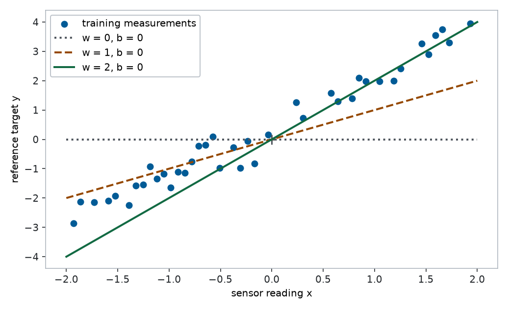
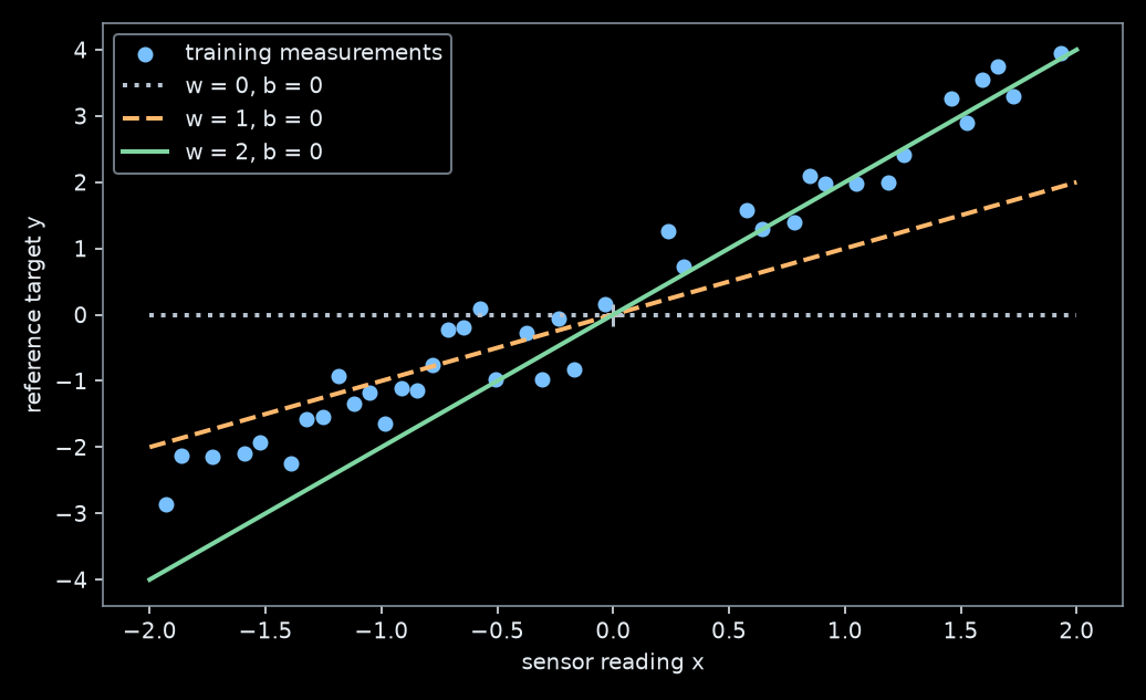
Discuss: can any choice of weight move the predicted value at \(x=0\) away from zero? If the sensor needs an offset, changing only the slope is insufficient. This is a limitation of the model family, not of your search strategy.

5.3.3 Add a bias — a second parameter

Give the model an adjustable offset \(b\), called a bias:

\[ \hat y^{(i)}=wx^{(i)}+b. \tag{5.3}\]

The weight sets the slope; the bias shifts every prediction by the same amount. This is conventionally called linear regression. More precisely, it is affine because its line need not pass through the origin. The model specifies predictions, but does not specify how to find its parameters.

5.3.4 Your second attempt — two parameters, 2 minutes

Before running the next cell, predict how increasing each parameter moves the line. Then try at most two parameter pairs. Record the values, the printed score, and the reason for your next change. The score averages squared prediction errors; smaller is better. We will now explain that score rather than accepting it as a black box.

A scatter plot of synthetic sensor readings and targets, with a candidate straight line and a horizontal training-mean baseline. — Figure 5.2: Your candidate calibration line and the training measurements. Change only the weight and bias to try a new fit.

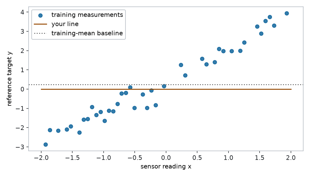
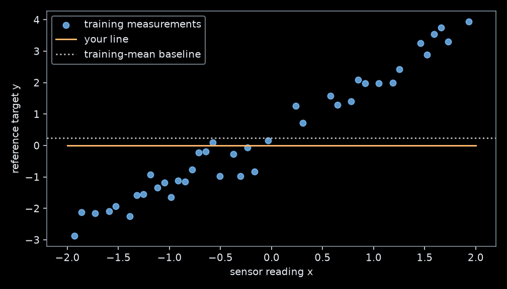
print(f"Your MSE: {score_try:.4f}; baseline MSE: {baseline_score:.4f}")

Your MSE: 3.7590; baseline MSE: 3.7026

Attempt	Weight \(w\)	Bias \(b\)	Score	Reason for the next change
1–2	Record your choices

Pause before reading on. What worked? Which change made the score worse? How do you know when to stop? If you already obtained a good fit, that is success: the difficulty is now explaining a reliable procedure that someone else could follow.

A grid search is one possible procedure: test ten values of each parameter. That needs \(10^2=100\) fits for two parameters. With twenty weights and one bias, the same approach needs \(10^{21}\) combinations. This count motivates a local rule that tells us which way to move. It does not prove that every search method is inefficient.

Keep an experiment record

Save your best pair as w_manual, b_manual in your notes. The later worked comparison uses a fixed example guess so that the published chapter is reproducible. Replace that guess with your own when comparing your attempts.

5.4 Understand: what exactly are we fitting?

5.4.1 Turn discrepancies into an objective

Define the residual as the observed value minus the prediction:

\[ r^{(i)} = y^{(i)}-\hat y^{(i)}. \]

Positive means underprediction; negative means overprediction. Simply adding signed errors would let them cancel. We instead square each one, giving the per-example loss \(\ell^{(i)}=(r^{(i)})^2\). For \(n\) training examples, define the objective

\[ L(w,b)=\frac{1}{n}\sum_{i=1}^{n}(y^{(i)}-(wx^{(i)}+b))^2. \tag{5.4}\]

This is mean squared error (MSE). The data are fixed when we optimize it; \(w\) and \(b\) are the variables. Squaring penalizes large discrepancies strongly: an error of 4 contributes sixteen times as much as an error of 1. That also makes this objective sensitive to outliers.

def mse(x_values, y_values, w, b):
    prediction = w * x_values + b
    assert prediction.shape == y_values.shape
    return ((y_values - prediction) ** 2).mean()

signed_errors = torch.tensor([-2.0, 2.0], dtype=DTYPE)
print("Mean signed error:", signed_errors.mean().item())
print("Mean squared error:", signed_errors.square().mean().item())
assert mse(x, y, w_try, b_try).item() == score_try

Mean signed error: 0.0
Mean squared error: 4.0

MSE has squared target units. Its square root, RMSE, has the original target units. Both order candidate predictions identically on the same dataset, but a numerical MSE value is not an error in original units.

5.4.2 Recall: a partial derivative changes one parameter

An ordinary derivative measures how a function changes when its one input changes. For \(L(w,b)\) there are two adjustable inputs. A partial derivative with respect to \(w\) changes \(w\) while holding \(b\) and every data value fixed. Similarly, \(\partial L/\partial b\) holds \(w\) fixed. Neither differentiates with respect to an observation \(x^{(i)}\).

Imagine slicing the two-dimensional loss surface at one fixed bias. Along that slice, the problem is a familiar function of one variable. The derivative is the tangent slope at the current weight.

Training MSE as a function of weight with bias fixed at zero. A tangent at weight 0.5 has negative slope and predicts a local loss decrease for a small positive weight change. — Figure 5.3: A partial derivative is the slope along one parameter direction while the other parameter stays fixed.

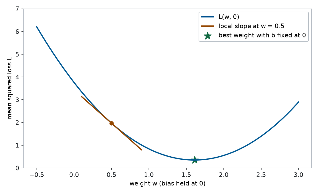
5.4.3 Derive the two partial derivatives

Ask first: what happens if we change the bias slightly while keeping the weight fixed? You already know the appropriate tool: \(\partial L/\partial b\).

For a single squared residual, the chain rule gives

\[ \frac{\partial}{\partial b}(y^{(i)}-(wx^{(i)}+b))^2 =2(y^{(i)}-(wx^{(i)}+b))\cdot(-1). \]

Differentiate the sum term by term:

\[ \boxed{\frac{\partial L}{\partial b}=-\frac{2}{n}\sum_{i=1}^{n}r^{(i)}}. \tag{5.5}\]

If the average residual is positive, the model underpredicts on average. Increasing \(b\) slightly decreases the loss. Increasing \(b\) is the promising move. The derivative is a local statement, so it does not tell us how far we can safely move.

Now hold \(b\) fixed and change \(w\). The inner derivative is \(-x^{(i)}\), giving

\[ \boxed{\frac{\partial L}{\partial w}=-\frac{2}{n}\sum_{i=1}^{n}r^{(i)}x^{(i)}}. \tag{5.6}\]

The weight derivative accounts for each reading’s sign and magnitude. You cannot infer it from the mean residual alone.

Mathematics bridge: a two-example calculation

Take \(x=(1,2)\), \(y=(2,3)\), and initially \(w=b=0\). Predictions are \((0,0)\), so residuals are \((2,3)\) and \(L=(4+9)/2=6.5\).

The bias derivative is \(-2(2+3)/2=-5\). The weight derivative is \(-2(2\cdot1+3\cdot2)/2=-8\). Both are negative: small increases in either parameter reduce the loss here. These are derivatives with respect to the parameters, not the slope of the fitted line with respect to \(x\).

5.4.4 Check the derivative independently

A numerical check changes one parameter by a tiny amount \(h\) and compares loss values. The central difference

\[ \frac{L(w+h,b)-L(w-h,b)}{2h}\approx\frac{\partial L}{\partial w} \]

should agree with our formula. It is a check at a chosen point, not a proof for all inputs. We use double precision and \(h=10^{-5}\); an extremely small \(h\) can amplify rounding error.

w_check, b_check, h = 0.3, -0.2, 1e-5
r_check = y - (w_check * x + b_check)
manual = torch.stack((-2 * (r_check * x).mean(), -2 * r_check.mean()))
finite_difference = torch.stack((
    (mse(x, y, w_check + h, b_check) - mse(x, y, w_check - h, b_check)) / (2 * h),
    (mse(x, y, w_check, b_check + h) - mse(x, y, w_check, b_check - h)) / (2 * h),
))
print("Partial derivatives [weight, bias]:", manual.tolist())
print("Finite differences:              ", finite_difference.tolist())
torch.testing.assert_close(manual, finite_difference, atol=1e-8, rtol=1e-8)

Partial derivatives [weight, bias]: [-3.3932375523672214, -0.9551973051374867]
Finite differences:               [-3.393237552384853, -0.9551973050969663]

5.4.5 Discuss fitting strategies before choosing one

Pairs, 3 minutes: propose a repeatable fitting procedure. What quantities will it inspect? Which parameter or parameters will it change? What would justify stopping? How could you tell that the procedure made things worse?

Possible proposals include a grid of candidate pairs, changing one coordinate at a time, following both derivatives, or solving all fitting equations together. Keep the model and loss fixed while comparing these procedures. A good manual guess is useful evidence, but it is not yet a general fitting rule.

5.4.6 Solve one coordinate at a time: coordinate descent

Instead of choosing a small step, we can minimize the loss exactly with respect to one parameter while holding the other fixed. Solving \(\partial L/\partial w=0\) at bias \(b_t\), then solving \(\partial L/\partial b=0\) using the new weight, gives

\[ \boxed{ w_{t+1}=\frac{\sum_i x^{(i)}(y^{(i)}-b_t)}{\sum_i(x^{(i)})^2}, \qquad b_{t+1}=\frac1n\sum_i\left(y^{(i)}-w_{t+1}x^{(i)}\right). } \tag{5.7}\]

The first denominator must be positive: at least one training input must be nonzero. Each of these one-variable objectives is a quadratic; setting its derivative to zero gives its minimum. The bias formula is simply the mean remaining offset after fitting the current weight.

These are sequential updates: the bias uses \(w_{t+1}\), not \(w_t\). This is called coordinate descent, since we minimize the loss. Coordinate ascent would maximize an objective. Each exact coordinate minimization leaves the full training MSE unchanged or reduces it, although one sweep need not reach the joint optimum.

w_coordinate, b_coordinate = 0.0, 0.0
coordinate_history = [mse(x, y, w_coordinate, b_coordinate).item()]
for sweep in range(5):
    w_coordinate = (x * (y - b_coordinate)).sum().item() / x.square().sum().item()
    coordinate_history.append(mse(x, y, w_coordinate, b_coordinate).item())
    b_coordinate = (y - w_coordinate * x).mean().item()
    coordinate_history.append(mse(x, y, w_coordinate, b_coordinate).item())
assert all(later <= earlier + 1e-12 for earlier, later in
           zip(coordinate_history, coordinate_history[1:]))
print("Coordinate descent [weight, bias]:", w_coordinate, b_coordinate)

Coordinate descent [weight, bias]: 1.655874390119084 0.4591479353135021

Check: why is the exact bias update not the same as taking a fixed small derivative step? For this quadratic problem we can solve the coordinate minimum. For many later neural-network parameters, that exact coordinate solve is unavailable.

5.4.7 A new object: the gradient vector

There is one partial derivative for every parameter. Put them in an ordered column, using the same order as the parameters:

\[ \boldsymbol{\theta}=\begin{bmatrix}w\\b\end{bmatrix}, \qquad \underbrace{\nabla L(\boldsymbol{\theta})}_{\text{gradient}} =\begin{bmatrix}\partial L/\partial w\\\partial L/\partial b\end{bmatrix}. \tag{5.8}\]

The symbol \(\nabla\) is pronounced “nabla”; \(\nabla L\) is read “gradient of \(L\).” The gradient is a vector because its two entries describe changes along two different parameter coordinates. It is not a new differentiation operation: we have already computed its entries.

At our two-example starting point, \(\nabla L=(-8,-5)^\top\). The superscript \(\top\) means transpose; it turns the displayed row into a column. Notice the roles: \(L\) is a single number, while its gradient has one number per parameter.

Why combine them? For small changes \(\Delta w\) and \(\Delta b\), the linear approximation is

\[ \Delta L\approx\frac{\partial L}{\partial w}\Delta w+ \frac{\partial L}{\partial b}\Delta b. \]

Choose each change as a small negative multiple of its derivative, with \(\eta>0\):

\[ \Delta w=-\eta\frac{\partial L}{\partial w},\qquad \Delta b=-\eta\frac{\partial L}{\partial b}. \]

Then the predicted change becomes

\[ \Delta L\approx-\eta\left[ \left(\frac{\partial L}{\partial w}\right)^2+ \left(\frac{\partial L}{\partial b}\right)^2\right]\leq0. \]

This explains the minus sign. In the current parameter coordinates, the negative gradient is the direction of steepest local decrease for a fixed, small Euclidean step length. A zero gradient gives no first-order direction; large steps are not covered by this approximation.

5.4.8 See the gradient in two-dimensional parameter space

The first plot has axes reading and target. This plot has axes weight and bias. Every point here specifies an entire candidate line; its contour value is the full training MSE. The arrows are evaluated at \((w,b)=(0,1.2)\) on the calibration training set, not on the separate two-example hand calculation. The gradient points toward steepest local increase; its negative points toward steepest local decrease, measured using Euclidean distance in the displayed parameter coordinates. The arrows show directions, not a recommended jump all the way to their tips.

Contours of training MSE over weight and bias. At the starting point, opposite arrows mark the gradient toward increasing loss and the negative gradient toward decreasing loss; the least-squares optimum is marked. — Figure 5.4: Opposite directions at the same parameter point: the gradient increases squared loss locally, and the negative gradient decreases it locally.

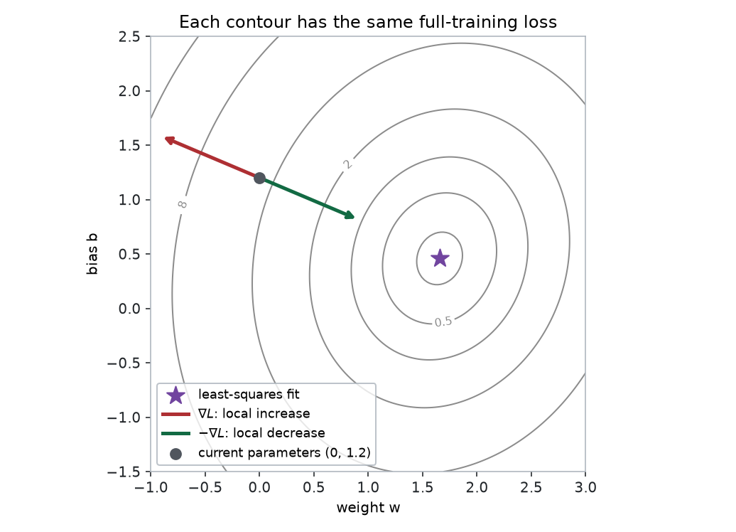
Predict: does the negative-gradient arrow point exactly at the optimum? Not necessarily: a local steepest direction need not be a direct route to the minimum. Changing feature scales changes the shape of these contours and the meaning of a fixed parameter-space step.

5.5 Fit one example first: stochastic gradient descent

Instead of averaging forty residuals immediately, select a single training pair \((x^{(i)},y^{(i)})\). Its squared loss and gradient are

\[ \ell^{(i)}(w,b)=(y^{(i)}-(wx^{(i)}+b))^2, \qquad \nabla\ell^{(i)}(w,b)=-2r^{(i)} \begin{bmatrix}x^{(i)}\\1\end{bmatrix}. \]

This uses exactly the same chain-rule calculation as before, with one residual and no average. A single-example gradient update is

\[ \boxed{ w_{t+1}=w_t+\eta\,2r_t^{(i)}x^{(i)}, \qquad b_{t+1}=b_t+\eta\,2r_t^{(i)}, \qquad r_t^{(i)}=y^{(i)}-(w_tx^{(i)}+b_t). } \tag{5.9}\]

Both derivatives use the old parameters. Repeatedly choosing examples at random and taking these steps is stochastic gradient descent (SGD). The learning rate \(\eta>0\) controls the step size. We choose it; it is a hyperparameter, rather than a parameter fitted by this rule.

5.5.1 One step by hand

Choose the example \(x^{(i)}=1\), \(y^{(i)}=2\), start at \(w=b=0\), and use \(\eta=0.1\). The residual is \(2\), the per-example gradient is \((-4,-4)^\top\), and the updated parameters are \((0.4,0.4)\). The selected example’s prediction becomes \(0.8\), so its loss falls from \(4\) to \(1.44\).

x_one, y_one = 1.0, 2.0
w_sgd, b_sgd, eta = 0.0, 0.0, 0.1
r_one = y_one - (w_sgd * x_one + b_sgd)
w_sgd, b_sgd = w_sgd + eta * 2 * r_one * x_one, b_sgd + eta * 2 * r_one
print("One-example update [weight, bias]:", w_sgd, b_sgd)
print("Selected-example loss:", (y_one - (w_sgd * x_one + b_sgd)) ** 2)

One-example update [weight, bias]: 0.4 0.4
Selected-example loss: 1.44

A sufficiently small negative-gradient step decreases the selected example’s loss when its gradient is nonzero. It does not guarantee a decrease in the full training objective. For example, take \(x=(0,0)\), \(y=(-1,1)\), and initially \(b=0\). The full MSE is already \(1\); a step of size \(0.1\) using only the target \(1\) changes \(b\) to \(0.2\). That example’s loss falls to \(0.64\), but full MSE rises to \(1.04\).

x_counter = torch.tensor([0.0, 0.0], dtype=DTYPE)
y_counter = torch.tensor([-1.0, 1.0], dtype=DTYPE)
assert mse(x_counter, y_counter, 0.0, 0.2) > mse(x_counter, y_counter, 0.0, 0.0)
assert (0.2 - 1.0) ** 2 < (0.0 - 1.0) ** 2

5.5.2 Why random examples can still fit the full dataset

At any fixed parameter pair, the average of all per-example gradients equals the gradient of MSE:

\[ \frac1n\sum_i\nabla\ell^{(i)}(w,b)=\nabla L(w,b). \]

If every example has the same chance of being selected, its sampled gradient has this average direction. In probability language, it is an unbiased estimate of the full gradient. An individual direction can disagree strongly with that average, so SGD paths fluctuate. This averaging statement applies at fixed parameters; it is not a claim that successive noisy updates exactly reproduce batch descent.

Here is the entire single-example mechanism with uniform sampling and a fixed seed:

w_stochastic, b_stochastic = 0.0, 0.0
sample_rng = torch.Generator().manual_seed(23)
sgd_history = [mse(x, y, w_stochastic, b_stochastic).item()]
for update in range(200):
    i = torch.randint(len(x), (1,), generator=sample_rng).item()
    residual_i = y[i].item() - (w_stochastic * x[i].item() + b_stochastic)
    dw_i = -2 * residual_i * x[i].item()
    db_i = -2 * residual_i
    w_stochastic, b_stochastic = w_stochastic - 0.03 * dw_i, b_stochastic - 0.03 * db_i
    sgd_history.append(mse(x, y, w_stochastic, b_stochastic).item())
assert sgd_history[-1] < sgd_history[0]
print("SGD final full-training MSE:", sgd_history[-1])

SGD final full-training MSE: 0.16101283947215972

These diagnostics evaluate full training MSE, so successive values describe the same objective. The loss of a different selected example on every update would mix different functions and be difficult to interpret. A fixed learning rate can leave fluctuations near the optimum; a decreasing schedule is one later refinement.

5.6 Average the examples: batch gradient descent

Now use every training example to compute each update direction. This is full-batch gradient descent; in this chapter “batch gradient descent” means that full-batch case. Its gradient is the average of the one-example derivatives that we have just implemented.

5.6.1 Repeat a simultaneous negative-gradient update

Gradient descent repeats three operations:

Compute predictions and residuals at the current parameters.
Compute all partial derivatives at those same parameters.
Subtract a small multiple of each derivative from its parameter.

The multiplier \(\eta\) is the learning rate. We choose it; training does not fit it in this procedure. It is therefore a hyperparameter. With \(t\) denoting an update number,

\[ w_{t+1}=w_t-\eta\frac{\partial L}{\partial w}(w_t,b_t),\qquad b_{t+1}=b_t-\eta\frac{\partial L}{\partial b}(w_t,b_t). \tag{5.10}\]

In vector notation this is simply \(\boldsymbol{\theta}_{t+1}=\boldsymbol{\theta}_t-\eta\nabla L(\boldsymbol{\theta}_t)\). Both versions describe the same calculation.

For the two-example calculation and \(\eta=0.1\), the new parameters are \(w=0.8\) and \(b=0.5\). Check the result rather than relying only on the arrow:

x_small = torch.tensor([1.0, 2.0], dtype=DTYPE)
y_small = torch.tensor([2.0, 3.0], dtype=DTYPE)
w_small, b_small = 0.0, 0.0
r_small = y_small - (w_small * x_small + b_small)
partial_w = -2 * (r_small * x_small).mean().item()
partial_b = -2 * r_small.mean().item()
w_new = w_small - 0.1 * partial_w
b_new = b_small - 0.1 * partial_b
print("Old MSE:", mse(x_small, y_small, w_small, b_small).item())
print("New parameters:", w_new, b_new)
print("New MSE:", mse(x_small, y_small, w_new, b_new).item())
assert abs(mse(x_small, y_small, w_new, b_new).item() - 0.65) < 1e-12

Old MSE: 6.5
New parameters: 0.8 0.5
New MSE: 0.6499999999999999

We computed both derivatives before changing either parameter. Recomputing the second derivative after the first change defines a different update rule.

5.7 Solve the same objective directly: least squares

All students should know what the reference does: find parameters minimizing the same sum of squared residuals, without taking the small iterative steps above. You do not need its derivation yet. Minimizing MSE and minimizing the sum of squares give the same parameters because \(n\) is fixed and positive.

With \(\mathbf A\) containing one row \([x^{(i)},1]\) per training example and \(\boldsymbol\theta=(w,b)^\top\), the direct problem is

\[ \boldsymbol\theta^*\in\operatorname*{arg\,min}_{\boldsymbol\theta} \|\mathbf A\boldsymbol\theta-\mathbf y\|_2^2. \tag{5.11}\]

The factor \(1/n\) does not change the minimizing parameters. A solver represents the bias by an extra column of ones. Each row [x_i, 1] multiplied by the column [w, b] gives w*x_i + b. This is a small first use of matrix notation, after we understand the scalar model.

# Shape: (40, 2) times (2, 1) gives 40 predictions with shape (40, 1).
design = torch.stack((x, torch.ones_like(x)), dim=1)
solution = torch.linalg.lstsq(design, y[:, None]).solution[:, 0]
w_ls, b_ls = solution.tolist()
print(f"Direct least squares: w={w_ls:.4f}, b={b_ls:.4f}")
print("Minimum training MSE:", mse(x, y, w_ls, b_ls).item())

Direct least squares: w=1.6559, b=0.4591
Minimum training MSE: 0.14230809498415092

The solver gives an independent reference for judging iterative procedures on this dataset. A minimum training score does not establish good performance on new data. For this small problem the direct solver is an excellent fitting method; we learn gradient descent because it also applies to later models without a comparable closed-form solution.

5.7.1 Compare paths without changing the objective

Training-MSE contours over weight and bias with coordinate-descent, batch-gradient, and stochastic-gradient paths from the same zero initialization, together with the direct least-squares optimum. — Figure 5.5: Different procedures fit the same affine model on the same training data. Coordinate steps move along one axis; batch steps use an averaged direction; single-example SGD fluctuates. The direct solver returns the minimum without this iterative path.

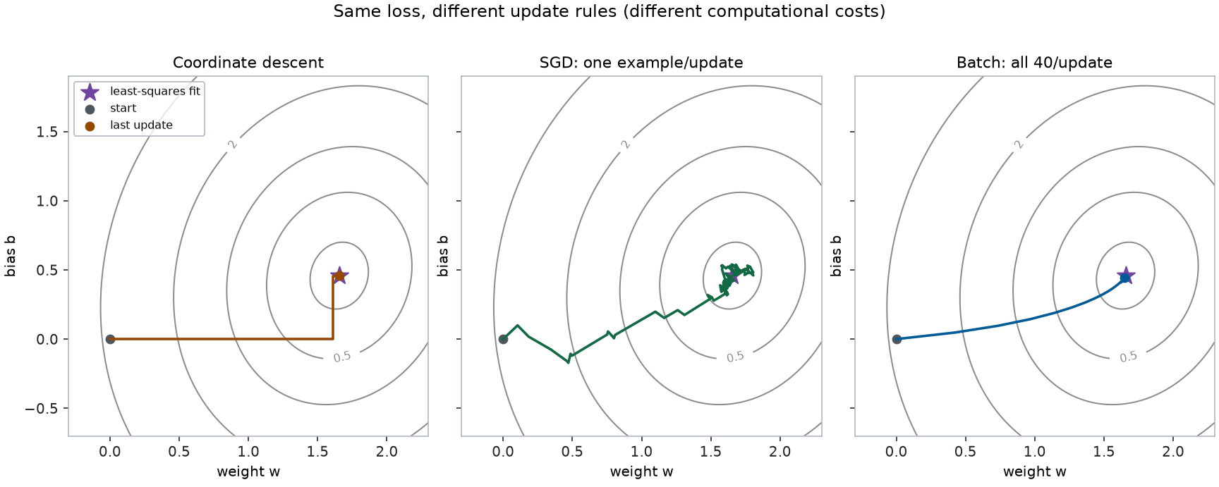
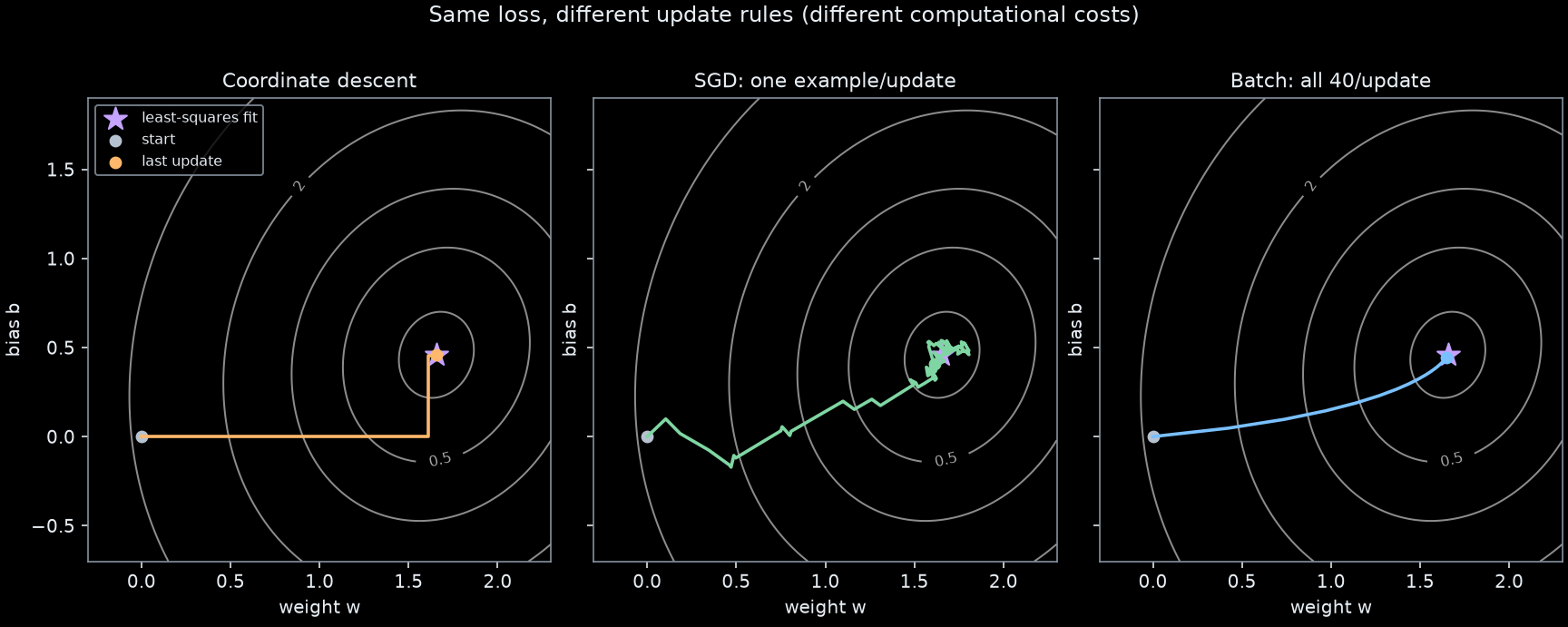
This is a comparison of mechanisms, not speed. A coordinate sweep, a batch update, and an SGD update use different amounts of work. The exercise asks you to state the budget before comparing final losses.

5.8 Improve: return to the calibration task

5.8.1 Replace guessing with repeated updates

Predict first: starting from the same zero parameters as the first attempt, what should happen to training MSE over 80 small updates? Must it reach zero, even with a correct algorithm?

The entire fitting mechanism is visible here. .item() turns a scalar tensor into a Python number. No regression helper or automatic differentiation is involved yet.

w, b = 0.0, 0.0
learning_rate = 0.1
history = [mse(x, y, w, b).item()]
parameter_path = [(w, b)]
for step in range(80):
    residual = y - (w * x + b)
    derivative_w = -2 * (residual * x).mean().item()
    derivative_b = -2 * residual.mean().item()
    w = w - learning_rate * derivative_w
    b = b - learning_rate * derivative_b
    history.append(mse(x, y, w, b).item())
    parameter_path.append((w, b))

assert history[-1] < history[0]
assert torch.isfinite(torch.tensor(history)).all()
print(f"Learned weight={w:.4f}, bias={b:.4f}, training MSE={history[-1]:.4f}")

Learned weight=1.6559, bias=0.4591, training MSE=0.1423

5.8.2 Check the iterative fit against the direct reference

print("MSE gap to reference:", mse(x, y, w, b).item() - mse(x, y, w_ls, b_ls).item())
torch.testing.assert_close(torch.tensor([w, b], dtype=DTYPE), solution,
                           atol=1e-6, rtol=1e-6)

MSE gap to reference: 2.0816681711721685e-15

Agreement is evidence that this batch-gradient run found the same training fit on these data. It does not test generalization or a different optimizer configuration.

Two panels show a fitted line following noisy training data and an MSE curve decreasing rapidly before reaching a nonzero plateau. — Figure 5.6: The iterative fit learns both parameters systematically. The right panel records loss after each update, including the initial loss at update zero.

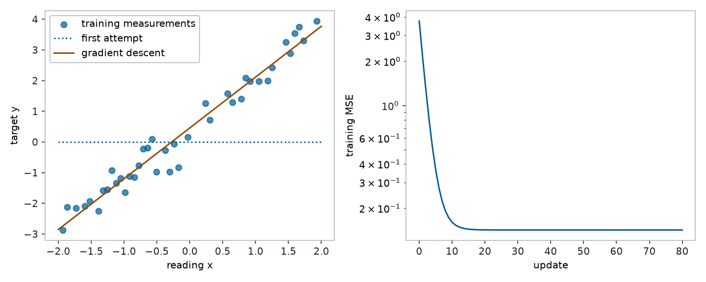
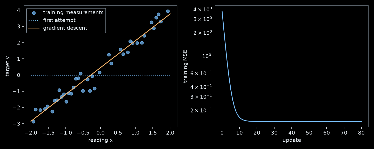
A small, nonzero loss is expected when a straight line cannot interpolate all noisy measurements. A plateau alone, however, does not establish that we have found the best line. Compare with the direct least-squares fit introduced above.

5.8.3 A deliberate failure: can a larger step be worse?

Controlled hypothesis: at a fixed update budget, an excessively large learning rate can increase loss even when the derivatives are correct. Keep the data, initial parameters, objective, and budget fixed; change only the learning rate.

Now that we have written the loop once, package it so each run resets its state. The safety stop records an unsuccessful run before values overflow; it is not a successful convergence criterion.

def fit_scalar(x_values, y_values, rate, steps=80):
    weight, bias = 0.0, 0.0
    losses = [mse(x_values, y_values, weight, bias).item()]
    for _ in range(steps):
        residual = y_values - (weight * x_values + bias)
        dw = -2 * (residual * x_values).mean().item()
        db = -2 * residual.mean().item()
        weight, bias = weight - rate * dw, bias - rate * db
        losses.append(mse(x_values, y_values, weight, bias).item())
        if not torch.isfinite(torch.tensor(losses[-1])) or losses[-1] > 1e12:
            return weight, bias, losses, "stopped: unstable"
    return weight, bias, losses, "budget completed"

runs = {rate: fit_scalar(x, y, rate) for rate in (0.005, 0.1, 1.0)}
for rate, (_, _, losses, status) in runs.items():
    print(f"rate={rate}: {status}; {len(losses)-1} updates; final MSE={losses[-1]:.4g}")

rate=0.005: budget completed; 80 updates; final MSE=0.6441
rate=0.1: budget completed; 80 updates; final MSE=0.1423
rate=1.0: stopped: unstable; 25 updates; final MSE=2.185e+12

Log-scale MSE curves for learning rates 0.005, 0.1, and 1.0. The moderate-rate curve falls fastest to low loss; the large-rate curve rises. — Figure 5.7: Only the learning rate changes. A small rate makes slow progress, a moderate rate approaches a plateau, and a large rate is unstable. Unstable runs may stop before the common maximum budget.

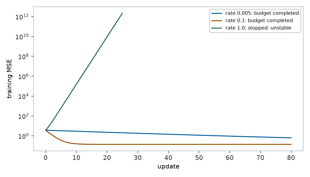
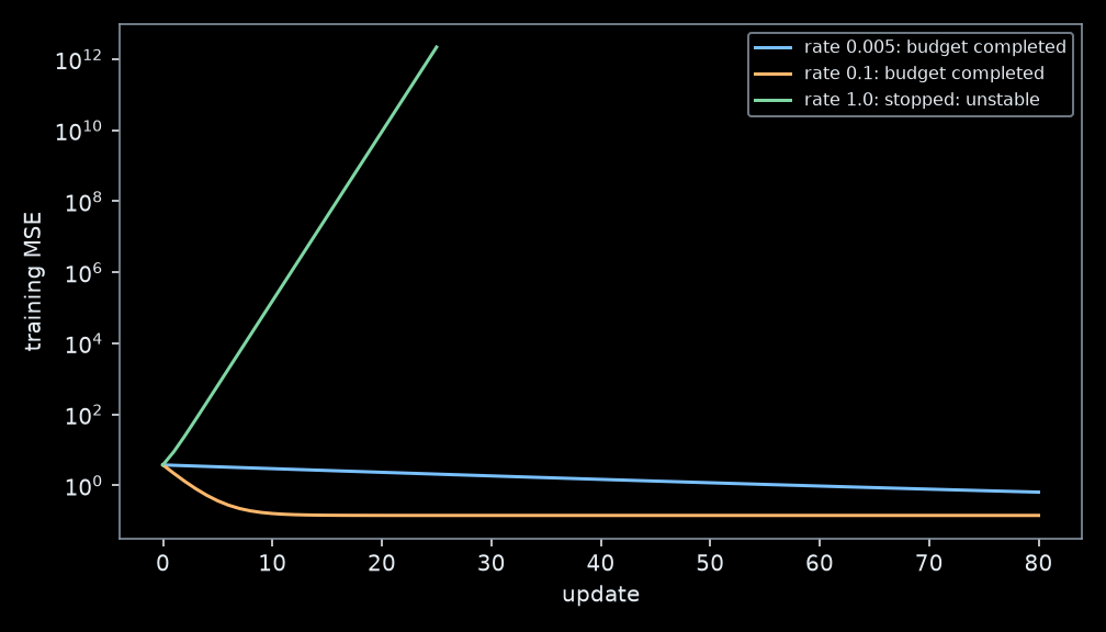
Core checkpoint. Explain this result using the word local. Which evidence points to an optimization problem rather than an unsuitable model? Choose a repair, state your prediction, then rerun. Compare your result with your first manual attempt; do not erase unsuccessful trials from your report.

5.8.4 Does it predict new measurements?

Training data determine the fitted parameters. Validation data help choose modeling and training settings. A test set is used after those choices are fixed. Repeatedly changing the model in response to the test score turns it into another validation set.

For this worked run, fix the model, rate 0.1, and 80 updates now. We diagnosed the optimizer on training loss. Use the validation score as a check before the final test report; in your own project, return to fitting if the check motivates a change, and keep test results hidden until you finish.

print(f"Validation MSE: {mse(x_valid, y_valid, w, b).item():.4f}")

Validation MSE: 0.0544

The next cell is the final evaluation. The baseline uses the training mean, even on the test set. This avoids fitting part of the evaluation procedure to the answers we are supposed to predict.

manual_w, manual_b = 1.0, 0.0  # Worked example; replace with your recorded first attempt.
models = {
    "training-mean baseline": (0.0, baseline),
    "manual example": (manual_w, manual_b),
    "gradient descent": (w, b),
    "direct least squares": (w_ls, b_ls),
}
print(f"{'method':26s} {'train MSE':>10s} {'test RMSE':>10s}")
for name, (weight, bias) in models.items():
    train_mse = mse(x, y, weight, bias).item()
    test_rmse = mse(x_test, y_test, weight, bias).sqrt().item()
    print(f"{name:26s} {train_mse:10.4f} {test_rmse:10.4f}")

method                      train MSE  test RMSE
training-mean baseline         3.7026     1.8157
manual example                 0.8388     0.9467
gradient descent               0.1423     0.4127
direct least squares           0.1423     0.4127

This small held-out sample gives a noisy estimate for new observations from the same generating process. It says little about a different sensor, a changed measurement process, or inputs far beyond the calibration range. Low training loss and reliable generalization are different claims.

5.9 Extend the same idea

5.9.1 Several inputs, one prediction

Suppose a second feature records temperature. For \(d\) features, put the measurements for example \(i\) in a vector \(\mathbf{x}^{(i)}\) and the weights in \(\mathbf w\). The model is still a weighted sum plus bias:

\[ \hat y^{(i)}=\sum_{j=1}^{d}w_j x_j^{(i)}+b. \]

The index \(j\) labels a feature; \(i\) still labels an example. Each weight gets its own familiar partial derivative:

\[ \frac{\partial L}{\partial w_j}=-\frac{2}{n}\sum_i r^{(i)}x_j^{(i)}. \]

Stack examples as rows of a matrix \(\mathbf X\) of shape \((n,d)\). Then

\[ \hat{\mathbf y}=\mathbf X\mathbf w+b\mathbf 1, \qquad \nabla_{\mathbf w}L=-\frac{2}{n}\mathbf X^\top\mathbf r. \]

Here \(\mathbf 1\) is a column of ones and \(\mathbf r\) is the residual column. The transpose swaps rows and columns. The matrix formula computes all the weight derivatives together; it does not change their definition. In code, use weights (d, 1) and targets (n, 1) to make this correspondence explicit. The lab introduces a shape error that would otherwise silently change the objective.

5.9.2 Between one example and all examples: minibatches

Our update averaged derivatives over every training example: full-batch gradient descent. A minibatch averages over a subset \(B\) instead:

\[ \frac{\partial L_B}{\partial w_j}=-\frac{2}{|B|}\sum_{i\in B}r^{(i)}x_j^{(i)}. \]

The expression is unchanged except for which examples enter the average. Random batches give different directions, so the full training loss need not decrease after every minibatch update. A batch of one is the smallest stochastic update; a batch containing the whole training set recovers full-batch descent.

An update changes parameters once. An epoch makes one pass through all training examples. With 40 examples and batches of 10, one epoch has four updates. A comparison must say whether it fixes epochs, updates, or another budget. You will make an equal-epoch comparison in the lab.

5.9.3 Let PyTorch compute the same derivatives

Automatic differentiation computes derivatives of the operations recorded in a computation graph. It does not know whether you intended the correct loss. First verify it on the derivatives we already understand:

w_auto = torch.tensor(0.3, dtype=DTYPE, requires_grad=True)
b_auto = torch.tensor(-0.2, dtype=DTYPE, requires_grad=True)
loss_auto = mse(x, y, w_auto, b_auto)
loss_auto.backward()
auto = torch.stack((w_auto.grad, b_auto.grad))
print("Automatic derivatives:", auto.tolist())
torch.testing.assert_close(auto, manual)

Automatic derivatives: [-3.3932375523672214, -0.9551973051374868]

.backward() computes derivatives; it does not update parameters. .grad stores them. In a training loop, gradients must be cleared before the next backward pass, because PyTorch otherwise adds them to existing values. The lab connects these operations to an explicit update, then to nn.Linear and torch.optim.SGD.

5.10 Depth choice: connect to Math 3

This section is optional. The common learning path above did not require likelihoods or a derivation of the least-squares formula.

5.10.1 Population risk: the goal beyond the recorded examples

If \(X,Y\) describe a new input/target pair from the intended measurement process, the population risk is

\[ R(w,b)=\mathbb E\left[(wX+b-Y)^2\right]. \]

The expectation \(\mathbb E\) means an average over possible new pairs. It is not the average over just the training rows, which is our empirical MSE \(L\). A held-out score estimates future error when its examples represent that intended process; a changed sensor or sampling process can invalidate that interpretation. We optimize the available empirical objective and check whether its predictor generalizes. No Gaussian assumption is needed to define either squared-error score.

5.10.2 Least squares and the normal equations

For the step-by-step one-feature and matrix derivations, including the conditions for a unique minimum, continue to Additional material: exact solutions and basis functions. That notebook also shows how fixed nonlinear features lead toward learned representations in DNNs.

Combine \(\mathbf w\) and \(b\) into \(\boldsymbol\theta\) and add a column of ones to \(\mathbf X\), giving \(\widetilde{\mathbf X}\). The objective is

\[ L(\boldsymbol\theta)=\frac1n\|\widetilde{\mathbf X}\boldsymbol\theta-\mathbf y\|_2^2. \]

The squared norm means the sum of squared entries. Setting every partial derivative to zero gives the normal equations

\[ \widetilde{\mathbf X}^{\top}\widetilde{\mathbf X}\boldsymbol\theta =\widetilde{\mathbf X}^{\top}\mathbf y. \]

Because this objective is convex, a stationary point is a global minimum. The minimizer is unique if the augmented design has full column rank. With redundant columns, fitted training predictions can be unique even when parameters are not. Use a least-squares solver rather than explicitly inverting \(\widetilde{\mathbf X}^{\top}\widetilde{\mathbf X}\).

This connects two familiar ideas: least squares specifies what to minimize; gradient descent specifies one way to minimize it. Gradient descent does not define a different regression model.

5.10.3 When does maximum likelihood give the same fit?

Assume conditionally independent targets with Gaussian noise of a common variance \(\sigma^2>0\):

\[ y^{(i)}=wx^{(i)}+b+\varepsilon^{(i)},\qquad \varepsilon^{(i)}\overset{\mathrm{iid}}\sim\mathcal N(0,\sigma^2). \]

At fixed \(\sigma\), the negative log likelihood is

\[ -\log p(\mathbf y\mid\mathbf x,w,b,\sigma) =\frac n2\log(2\pi\sigma^2) +\frac{1}{2\sigma^2}\sum_i(y^{(i)}-wx^{(i)}-b)^2. \]

The first term does not depend on \(w,b\) and the multiplier on the sum is positive. Thus likelihood maximization and squared-error minimization choose the same parameters under these assumptions. MSE can still be used without assuming Gaussian noise; the likelihood interpretation then needs separate justification.

sigma = 0.35
candidates = torch.tensor([[0.0, 0.0], [1.0, 0.0], [w_ls, b_ls]], dtype=DTYPE)
errors = y - (candidates[:, :1] * x + candidates[:, 1:])
mse_values = errors.square().mean(dim=1)
# Evaluate the Gaussian density's log probability independently.
distribution = torch.distributions.Normal(
    candidates[:, :1] * x + candidates[:, 1:], sigma
)
negative_log_likelihood = -distribution.log_prob(y).sum(dim=1)
constant = len(x) / 2 * torch.log(torch.tensor(2 * torch.pi * sigma**2, dtype=DTYPE))
torch.testing.assert_close(negative_log_likelihood,
                           constant + len(x) * mse_values / (2 * sigma**2))
print("MSE ranking:", torch.argsort(mse_values).tolist())
print("NLL ranking:", torch.argsort(negative_log_likelihood).tolist())

MSE ranking: [2, 1, 0]
NLL ranking: [2, 1, 0]

5.11 Knowledge checks — Core

Answer before consulting an instructor or an AI tool. These are formative checks; answers are in the instructor guide.

Which two quantities change during training, and which measured quantities remain fixed?
For \(x=(1,2)\) and \(y=(2,3)\) at \(w=1,b=0\), calculate MSE, both partial derivatives, and one update with \(\eta=0.1\).
What information does a gradient contain that a loss value alone does not? Why must its entry order match the parameter order?
A correct gradient followed by a large update increases loss. Which argument above explains why this is possible?
Training loss is low but held-out loss is high. Is reducing the learning rate necessarily the appropriate repair? Explain.
With 120 examples and batches of 20, how many updates are in five epochs?
Why can two methods agree on training MSE without proving that the prediction rule will work after the sensor changes?
Why does the exact bias update in coordinate descent use the newly solved weight? What guarantee does each coordinate solve give?
Give an example in which reducing one example’s loss increases full training MSE. Why does random single-example sampling still connect to the full gradient?
Which model limitation did adding the bias repair? Why could more careful fitting of the one-parameter model not repair it?

5.12 Summary

You first identified a supervised regression problem and tried a line with one adjustable weight. Adding a bias allowed an offset. A loss made those attempts comparable. Familiar partial derivatives supplied local information about each parameter; collecting them gave the gradient. Coordinate descent solved one parameter at a time. SGD used one example at a time; batch descent averaged their derivatives. Direct least squares solved the same fitting problem without small steps, while the learning-rate experiment exposed the limit of taking a local direction too far.

Keep these roles separate:

Component	This chapter
Data pipeline	Fixed split; training measurements used for fitting
Model / architecture	Weighted input plus bias
Objective	Mean squared training error
Optimizer	Coordinate descent, SGD, batch descent, or a direct least-squares solve
Evaluation	Training diagnostics, validation checks, final held-out RMSE

Optional continuation: closed-form least squares and basis functions develops the exact solution, diagnoses a best-fitting line with the wrong shape, and connects fixed features to neural networks.

Next, complete the lab: transfer the mechanism to two features, inspect a broadcasting failure, and repair a feature-scale problem. For support, use Python and tensors, linear algebra, or automatic differentiation.

Further reading: Zhang et al. (2023), Chapter 3, offers a complementary treatment of linear regression. This chapter’s experiment sequence, explanations, and figures are newly authored; the book’s attribution register records its earlier D2L connection.