9 Week 2 Lab: Logistic Regression – Deep Learning: Models, Training, and Adaptation

9.1 Lab contract

Continue the try → understand → improve cycle from the chapter. This notebook runs independently, from top to bottom, in the book environment. Use only concavity_mean and texture_mean as WDBC predictors. Do not inspect the reserved test data until the final checkpoint.

Common core: checkpoints 1–4 and the final evaluation. Short extensions for W02-02 and W02-03: checkpoints 5–6 on multiclass losses and shrinkage. Depth choice: the IRLS derivation. Budget about 3–4 hours including interpretation; divide the optional mathematical work within pairs if time is limited.

Before running

Write your predictions. Which will change when you standardize the features: correlation, the best achievable log loss, or GD’s trajectory? Which will change when you replace GD with Newton? What will count as evidence against your prediction?

9.2 1. Reproduce and audit the data pipeline — Core, 15 minutes

The helper functions below package the mechanisms already shown inline in the chapter. Read src/dlbook/logistic.py if you need to inspect them. All optimizers use float64, zero initialization, full batches, and mean log loss. The dataset and split are identical to the chapter.

import numpy as np
import matplotlib.pyplot as plt
from dlbook.plotting import show_plot
import torch
from torch import nn

from dlbook.logistic import (
    binary_metrics, design, gradient, gradient_descent, hessian,
    load_wdbc, loss, newton, sigmoid, stratified_split,
)

X_all, y_all = load_wdbc()
train, valid, test = stratified_split(y_all, seed=8)
X, y = X_all[train], y_all[train]
X_valid, y_valid = X_all[valid], y_all[valid]
mu, scale = X.mean(axis=0), X.std(axis=0)
Z, Z_valid = (X - mu) / scale, (X_valid - mu) / scale
A, B, B_valid = design(X), design(Z), design(Z_valid)
assert X.shape == (341, 2) and B.shape == (341, 3)
assert y.shape == (341,)  # A column vector would silently broadcast incorrectly.
assert set(train).isdisjoint(valid) and set(train).isdisjoint(test)
assert set(valid).isdisjoint(test)
assert len(np.unique(np.concatenate((train, valid, test)))) == len(y_all)
np.testing.assert_allclose(Z.mean(axis=0), 0, atol=1e-14)
np.testing.assert_allclose(Z.std(axis=0), 1, atol=1e-14)
assert np.isfinite(X_all).all() and set(np.unique(y_all)) == {0, 1}
print("Split sizes:", len(train), len(valid), len(test))
print("Training label counts:", np.bincount(y.astype(int)))
print("Training correlation:", np.corrcoef(X.T)[0, 1])

Split sizes: 341 113 115
Training label counts: [214 127]
Training correlation: 0.3407565373984516

Explain. Why does computing mu before splitting leak information, even if you do not use test labels? Why must you reuse the training mean and standard deviation on validation examples instead of fitting a new scaler there?

9.3 2. Check the mechanism against PyTorch — Core, 25 minutes

9.3.1 Predict the bug

A student writes the following training loss:

probabilities = torch.sigmoid(model(features))
loss = nn.BCEWithLogitsLoss()(probabilities, labels)

Explain the problem before running a corrected implementation. The function name says it expects logits. Also check shapes: (n, 1) and (n,) are not interchangeable just because both hold \(n\) values.

9.3.2 Verify the loss, gradient, and Hessian at a nonzero point

Using a nonzero parameter vector matters: an implementation can accidentally pass a check at a symmetric initialization and fail elsewhere.

Bt = torch.tensor(B, dtype=torch.float64)
yt = torch.tensor(y, dtype=torch.float64)
theta_probe = np.array([-0.4, 0.7, -0.2])
tt = torch.tensor(theta_probe, dtype=torch.float64, requires_grad=True)


def torch_objective(parameters):
    logits = Bt @ parameters
    assert logits.shape == yt.shape
    return nn.functional.binary_cross_entropy_with_logits(logits, yt)


jt = torch_objective(tt)
gt, = torch.autograd.grad(jt, tt)
Ht = torch.autograd.functional.hessian(torch_objective, tt)
np.testing.assert_allclose(jt.item(), loss(B, y, theta_probe), atol=1e-12)
np.testing.assert_allclose(gt.detach().numpy(), gradient(B, y, theta_probe), atol=1e-12)
np.testing.assert_allclose(Ht.detach().numpy(), hessian(B, theta_probe), atol=1e-12)
assert np.linalg.eigvalsh(hessian(B, theta_probe)).min() > 0
print("Scratch and PyTorch agree on the loss and both derivative orders.")

Scratch and PyTorch agree on the loss and both derivative orders.

9.3.3 Map the parameters to a standard model

theta_mle, newton_history, step_sizes = newton(B, y)
model = nn.Linear(2, 1, dtype=torch.float64)
with torch.no_grad():
    model.bias.copy_(torch.tensor(theta_mle[:1]))
    model.weight.copy_(torch.tensor(theta_mle[1:]).reshape(1, 2))
    logits = model(torch.tensor(Z, dtype=torch.float64)).squeeze(1)
np.testing.assert_allclose(logits.numpy(), B @ theta_mle, atol=1e-12)
print("Mapped nn.Linear loss:", nn.BCEWithLogitsLoss()(logits, yt).item())

Mapped nn.Linear loss: 0.262413276051727

For a standard GD implementation, use torch.optim.SGD, call zero_grad(), form logits, call the loss, then backward() and step(). Coding exercise: reproduce 100 standardized NumPy updates with PyTorch and compare final logits, using exactly the same initial parameters and \(\eta=1/\lambda_{\max}(B^\top B/(4n))\). Do not change the optimizer to Adam in this equivalence check.

9.4 3. Isolate scale and correlation — Core, 35 minutes

9.4.1 First, reproduce the coordinate comparison

Field	Predeclared choice
Hypothesis	Standardization helps GD; Newton needs fewer updates on this small problem.
Independent variables	Coordinates (raw/standardized), optimizer (GD/Newton)
Fixed controls	Rows, labels, model family, unpenalized mean log loss, initial logits zero
GD rule	\(\eta=1/L\) in each coordinate system; 2,000-update cap
Newton rule	Solve using curvature at every update; backtracking; decrement/2 \(\leq10^{-10}\)
Common comparison target	First loss gap to the stationary reference \(\leq10^{-6}\)
Primary evidence	Loss-gap trajectories and updates to the common target
Limits	One fixed split; update counts are not equal compute or elapsed time

reference = loss(B, y, theta_mle)
for name, matrix in [("raw", A), ("standardized", B)]:
    gd_theta, gd_history = gradient_descent(matrix, y, steps=2000)
    nt_theta, nt_history, _ = newton(matrix, y)
    for method, history in [("GD", gd_history), ("Newton", nt_history)]:
        reached = np.flatnonzero(history - reference <= 1e-6)
        first = str(reached[0]) if len(reached) else ">2000"
        print(f"{name:12s} {method:6s}: final={history[-1]:.6f}, updates to target={first}")
    np.testing.assert_allclose(matrix @ nt_theta, B @ theta_mle, atol=1e-8)

raw          GD    : final=0.628918, updates to target=>2000
raw          Newton: final=0.262413, updates to target=5
standardized GD    : final=0.262413, updates to target=80
standardized Newton: final=0.262413, updates to target=5

9.4.2 Now make correlation a controlled intervention

The original features are only moderately correlated. To test a stronger correlation effect without inventing new measurements or changing the model family, form an invertible coordinate transformation of the standardized training features:

\[ u=\widetilde x_1,\qquad v=\widetilde x_1+0.08\widetilde x_2. \]

You can recover \(\widetilde x_2=(v-u)/0.08\), so no predictive information is removed. Both new columns have standard deviations near one, but they are nearly redundant: their correlation is about \(0.997\). These are deliberately transformed coordinates, not a claim about the native UCI features. The transformation is specified in advance and uses no labels.

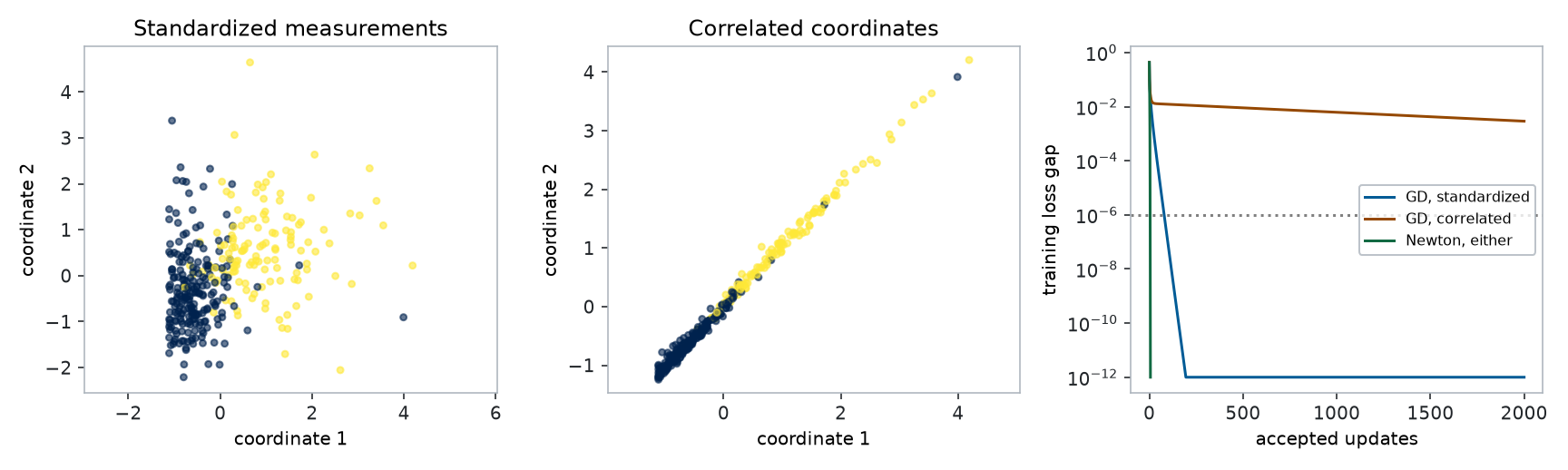
transform = np.array([[1.0, 1.0], [0.0, 0.08]])
Z_correlated = Z @ transform
C = design(Z_correlated)
print("Standard deviations:", Z_correlated.std(axis=0))
print("Correlation:", np.corrcoef(Z_correlated.T)[0, 1])
print("Initial Hessian condition number:", np.linalg.cond(hessian(C, np.zeros(3))))

theta_gd_z, h_gd_z = gradient_descent(B, y, steps=2000)
theta_gd_c, h_gd_c = gradient_descent(C, y, steps=2000)
theta_nt_c, h_nt_c, _ = newton(C, y)
np.testing.assert_allclose(C @ theta_nt_c, B @ theta_mle, atol=1e-8)
np.testing.assert_allclose(h_nt_c, newton_history, atol=1e-12)
print("Standardized GD final gap:", h_gd_z[-1] - reference)
print("Correlated-coordinate GD final gap:", h_gd_c[-1] - reference)

Standard deviations: [1.         1.03001022]
Correlation: 0.9973304211836751
Initial Hessian condition number: 748.8379358292657
Standardized GD final gap: -4.996003610813204e-16
Correlated-coordinate GD final gap: 0.002899312611917393

Left: standardized feature cloud; middle: strongly correlated transformed feature cloud with similar axis scales; right: log loss gap versus updates, showing slower GD in the correlated coordinates and overlapping fast Newton fits. — Figure 9.1: A controlled, invertible transformation makes the same two features nearly redundant while keeping their scales similar. GD slows down; Newton reaches the same fitted logits. All runs minimize unpenalized training log loss.

Interpretation, 150–200 words. Use the two interventions to distinguish scale, correlation, and curvature. Explain why it would be misleading to blame the original severe slowdown entirely on correlation. Explain why the matching Newton logits matter more than matching coefficient values across coordinate systems.

Stretch: repeat with transformation constants \(0.4\), \(0.2\), and \(0.1\), changing only this constant. Report the condition number and gap after the same GD budget. A nearly singular transformation will eventually cause numerical difficulties even for Newton; its theoretical coordinate invariance is an exact-arithmetic statement.

9.5 4. Evaluate probabilities and decisions — Core, 25 minutes

Freeze the primary model as the unpenalized two-feature MLE and its threshold as \(0.5\). This is the model we will assess on the test set at the end. The validation checks below diagnose it; they do not trigger changes to that predeclared primary model.

For probabilities \(p_i\) and labels \(y_i\):

Log loss averages \(-[y_i\log p_i+(1-y_i)\log(1-p_i)]\).
Brier score averages \((p_i-y_i)^2\); lower is better.
AUROC is the probability that a randomly drawn positive ranks above a randomly drawn negative, with half credit for ties.
Sensitivity is \(TP/(TP+FN)\); specificity is \(TN/(TN+FP)\).

The small helper uses pairwise comparisons for AUROC. This is transparent for 113 examples, though a sorting-based method is preferable for large datasets. Here positive always means malignant.

p_valid = sigmoid(B_valid @ theta_mle)
p_baseline = np.full(len(y_valid), y.mean())
for name, probabilities in [("training-prevalence baseline", p_baseline), ("logistic MLE", p_valid)]:
    print(name, {key: round(value, 4) for key, value in binary_metrics(y_valid, probabilities).items()})
for threshold in (0.3, 0.5, 0.7):
    metrics = binary_metrics(y_valid, p_valid, threshold=threshold)
    print(f"threshold {threshold:.1f}: sensitivity={metrics['sensitivity']:.3f}, "
          f"specificity={metrics['specificity']:.3f}")

training-prevalence baseline {'log_loss': 0.6598, 'accuracy': 0.6283, 'sensitivity': 0.0, 'specificity': 1.0, 'auroc': 0.5, 'brier': 0.2335}
logistic MLE {'log_loss': 0.3491, 'accuracy': 0.8761, 'sensitivity': 0.7619, 'specificity': 0.9437, 'auroc': 0.938, 'brier': 0.0961}
threshold 0.3: sensitivity=0.810, specificity=0.887
threshold 0.5: sensitivity=0.762, specificity=0.944
threshold 0.7: sensitivity=0.667, specificity=0.958

9.5.1 Calibration is a separate question

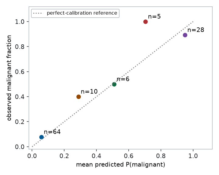
Group validation predictions into five fixed probability bins. Within each nonempty bin, compare the average prediction with the observed malignant fraction. Show the count: a point based on very few examples is weak evidence. A good-looking small-sample plot does not establish calibration in a new population.

Observed malignant fraction versus mean predicted probability in five fixed bins, with a diagonal reference and counts annotated beside each nonempty bin. — Figure 9.2: Validation reliability plot for the frozen unpenalized model. Counts beside the points reveal the small amount of evidence in some probability bins; empty bins are omitted.

Explain. Why can accuracy conceal poor sensitivity in an imbalanced dataset? Why is an AUROC above \(0.9\) not evidence that the probabilities are calibrated? Why should the test set not be used to choose a threshold?

9.6 5. Short extension: from two classes to several — W02-02, 20 minutes

WDBC has exactly two labels. Do not manufacture a third diagnosis. Use this separate tiny synthetic three-class example to learn the multiclass computation.

For \(K\) classes, compute one score \(z_k\) per class and use

\[ p_k=\frac{e^{z_k}}{\sum_j e^{z_j}},\qquad \ell(\boldsymbol z,y)=-z_y+\operatorname{logsumexp}(\boldsymbol z). \]

Subtracting the maximum score before exponentiating keeps the probabilities stable. Adding a constant to every score leaves softmax unchanged. For two scores \((0,z)\), softmax’s second probability equals \(\sigma(z)\).

synthetic_X = torch.tensor([[-2., 0.], [-1., 0.5], [2., 0.], [1., 0.5],
                            [0., 2.], [0.5, 1.5]], dtype=torch.float64)
synthetic_y = torch.tensor([0, 0, 1, 1, 2, 2], dtype=torch.long)
multiclass = nn.Linear(2, 3, dtype=torch.float64)
with torch.no_grad():
    multiclass.weight.zero_()
    multiclass.bias.zero_()
optimizer = torch.optim.SGD(multiclass.parameters(), lr=0.2)
for _ in range(150):
    optimizer.zero_grad()
    scores = multiclass(synthetic_X)
    objective = nn.CrossEntropyLoss()(scores, synthetic_y)  # Scores, not softmax outputs.
    objective.backward()
    optimizer.step()
with torch.no_grad():
    scores = multiclass(synthetic_X)
    manual_ce = (torch.logsumexp(scores, dim=1) - scores[torch.arange(6), synthetic_y]).mean()
    torch.testing.assert_close(manual_ce, nn.CrossEntropyLoss()(scores, synthetic_y))
    torch.testing.assert_close(torch.softmax(scores + 1000, dim=1), torch.softmax(scores, dim=1))
    assert (scores.argmax(dim=1) == synthetic_y).all()
z = torch.tensor([-1000., 0., 1000.], dtype=torch.float64)
torch.testing.assert_close(torch.softmax(torch.stack((torch.zeros_like(z), z), dim=1), dim=1)[:, 1],
                           torch.sigmoid(z))
print("Multiclass training log loss:", manual_ce.item())

Multiclass training log loss: 0.07517315940622242

This is an implementation and invariance check, not a generalization experiment. Explain why multiclass targets are integer class indices, whereas the binary loss uses floating-point zeros and ones.

9.7 6. Short extension: L1 and L2 change the objective — W02-03, 35 minutes

Return to WDBC and keep standardized coordinates fixed. Compare

\[ J_{L2}(b,\boldsymbol w)=J(b,\boldsymbol w)+\frac\lambda2\|\boldsymbol w\|_2^2, \qquad J_{L1}(b,\boldsymbol w)=J(b,\boldsymbol w)+\lambda\|\boldsymbol w\|_1. \]

Do not penalize the intercept. These are penalized objectives, not the unpenalized MLE used in the optimizer comparison. Standardization now also determines the meaning of a common penalty across features.

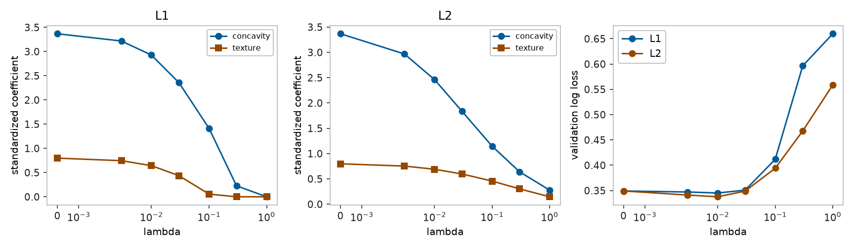
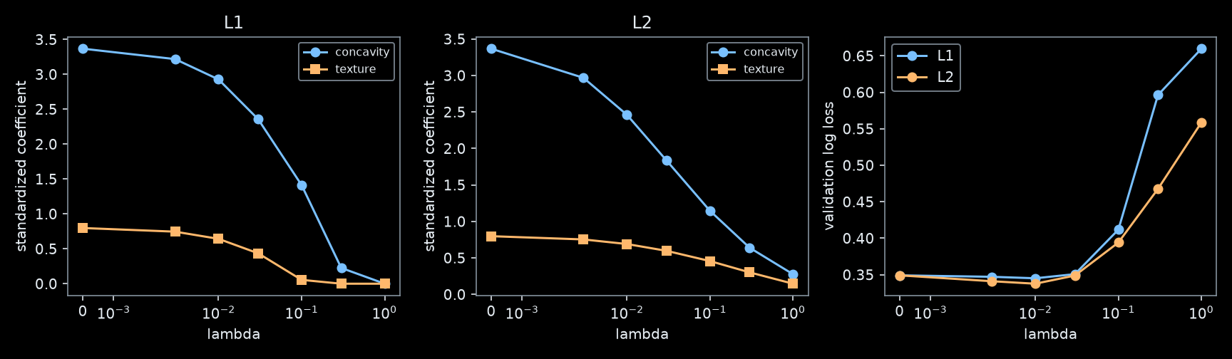
For L2, add \(\lambda\boldsymbol w\) to the weight gradient. Its smooth penalty usually reduces coefficient magnitudes without making them exactly zero. For L1, the derivative is not defined at zero; use a proximal step: first take a loss-gradient step, then apply soft thresholding

\[ w_j\leftarrow\operatorname{sign}(v_j)\max(|v_j|-\eta\lambda,0). \]

This explicitly sets small weights to zero. We compare objective-appropriate first-order solvers here; ordinary smooth Newton is not directly applicable to the L1 kink. With correlated features, individual coefficient magnitudes need not decrease monotonically along either path.

def fit_penalized(matrix, targets, penalty, strength, max_steps=10000):
    theta = np.zeros(matrix.shape[1])
    L = np.linalg.eigvalsh(matrix.T @ matrix / (4 * len(targets)))[-1]
    eta = 1 / (L + (strength if penalty == "L2" else 0))
    for _ in range(max_steps):
        g = gradient(matrix, targets, theta)
        if penalty == "L2":
            g[1:] += strength * theta[1:]
        candidate = theta - eta * g
        if penalty == "L1":
            candidate[1:] = np.sign(candidate[1:]) * np.maximum(np.abs(candidate[1:]) - eta * strength, 0)
        # Proximal-gradient mapping (ordinary gradient for L2).
        residual = np.max(np.abs(candidate - theta)) / eta
        theta = candidate
        if residual <= 1e-8:
            return theta
    raise RuntimeError("Penalized solver did not converge.")


strengths = np.array([0.0, 0.003, 0.01, 0.03, 0.1, 0.3, 1.0])
paths, validation_losses = {}, {}
for penalty in ("L1", "L2"):
    paths[penalty] = np.array([fit_penalized(B, y, penalty, s) for s in strengths])
    validation_losses[penalty] = np.array([loss(B_valid, y_valid, t) for t in paths[penalty]])
    np.testing.assert_allclose(B @ paths[penalty][0], B @ theta_mle, atol=2e-6)
    selected = np.argmin(validation_losses[penalty])
    print(penalty, "validation-selected lambda:", strengths[selected],
          "validation log loss:", round(validation_losses[penalty][selected], 4),
          "nonzero weights:", np.count_nonzero(paths[penalty][selected, 1:]))
assert np.count_nonzero(paths["L1"][-1, 1:]) == 0

L1 validation-selected lambda: 0.01 validation log loss: 0.3451 nonzero weights: 2
L2 validation-selected lambda: 0.01 validation log loss: 0.3377 nonzero weights: 2

Three panels show coefficient paths for L1 and L2 over increasing lambda, followed by validation log loss for both penalties. The intercept is excluded from the coefficient plots and from the penalties. — Figure 9.3: Controlled L1 and L2 paths: same standardized inputs, split, unpenalized validation metric, and convergence criterion. L1 produces exact zeros; L2 shrinks smoothly. The final panel compares validation log loss, not the penalized training objective.

Explain. Record one lambda with an exact L1 zero and compare the L2 coefficient there. Does a sparse coefficient establish that a measurement is causally irrelevant? Why is comparing the two penalized training objectives not a fair way to select the penalty? Would Newton and GD necessarily give different predictions after both fully minimize the same L2 objective?

9.8 Final checkpoint: open the test set once

The primary model and threshold were frozen in checkpoint 4. The regularization paths above are a separate validation exercise; they do not replace the primary model after looking at test results. Report this one assessment without tuning further. If you design a follow-up study, reserve new evaluation data.

X_test, y_test = X_all[test], y_all[test]
B_test = design((X_test - mu) / scale)
p_test = sigmoid(B_test @ theta_mle)
print("Frozen unpenalized MLE, test metrics:")
print({key: round(value, 4) for key, value in binary_metrics(y_test, p_test).items()})
pred = p_test >= 0.5
confusion = np.array([[np.sum((y_test == 0) & ~pred), np.sum((y_test == 0) & pred)],
                      [np.sum((y_test == 1) & ~pred), np.sum((y_test == 1) & pred)]])
print("Confusion matrix: rows true [benign, malignant], columns predicted [benign, malignant]")
print(confusion)

Frozen unpenalized MLE, test metrics:
{'log_loss': 0.3883, 'accuracy': 0.8348, 'sensitivity': 0.7209, 'specificity': 0.9028, 'auroc': 0.9273, 'brier': 0.1094}
Confusion matrix: rows true [benign, malignant], columns predicted [benign, malignant]
[[65  7]
 [12 31]]

A single fixed test split gives a reproducible classroom result, not a precise estimate of deployment performance or a population-wide medical claim. A follow-up analysis would need an appropriate sampling design, uncertainty estimates, and external evaluation.

9.9 Submission

Submit the runnable notebook and a concise report containing:

Your original predictions and what changed after the experiments.
The derivative checks and the shape of each major array.
A convergence comparison that distinguishes feature scaling from correlation, and updates from compute cost.
Validation and frozen-model test metrics with the positive class and threshold stated.
The multiclass invariance check and a controlled L1/L2 path comparison.
An individual explanation of why logistic MLE has no general closed-form solution and how a second-order iteration improves this example.

Math bridge: derive one Hessian entry, such as \(H_{12}\), directly from the scalar gradient. Coding bridge: annotate every line of the Newton loop with input and output shapes. Stretch: verify one Newton step using weighted least squares, and explain why those weights must change on the next iteration.