Try a classifier, understand likelihood, improve the optimizer
TipYour route through the chapter
Try → understand → improve. First, predict a binary label using two measurements and try the gradient-descent recipe from Week 1. Observe what is still going wrong. Then build a probability model, derive its objective, and use first and second derivatives to improve the same fit.
When
What you do
Before Session 1
Recall an affine predictor, a partial derivative, and one gradient-descent update from Week 1.
Session 1, 90 minutes
Try a classifier; observe slow fitting; derive sigmoid, likelihood, and the gradient.
Between sessions
Check one derivative and rerun the feature-scaling comparison, about 30 minutes.
Session 2, 90 minutes
Explain curvature; implement Newton’s method; compare convergence; start the lab.
After Session 2
Finish the lab, including the short multiclass and shrinkage extensions, about 3–4 hours.
The cells run in order on CPU in the book’s Python environment. A small attributed data subset is bundled with the repository; no download is needed during class. NumPy makes the small linear systems visible, and the lab checks the same computation with PyTorch. A rendered page shows results; change cells in a notebook or Quarto editor.
8.1 Starting points and learning outcomes
We use partial derivatives and the chain rule from Math 2, plus the gradient vector and gradient descent introduced in Week 1. The Hessian, which collects second partial derivatives, is new. Maximum likelihood is developed from an example; Math 3 is helpful but not required.
W02-01: Distinguish scores, probabilities, decisions, and losses in classification.
W02-02: Implement numerically stable binary and multiclass cross-entropy.
W02-03: Explain L1 sparsity and L2 shrinkage through regularization paths.
W02-04: Evaluate discrimination, probabilistic quality, and calibration.
Common core: binary logistic regression, likelihood, gradient descent, scaling, and a small Newton solve. Math bridge: scalar derivatives before matrix notation. Coding bridge: explicit shapes and executable checks. Depth choice:iteratively reweighted least squares (IRLS). The lab retains this week’s multiclass and regularization outcomes without interrupting the main optimization story.
8.2 Try: can two measurements predict a label?
The UCI Wisconsin Diagnostic Breast Cancer dataset contains measurements derived from images of fine-needle aspirates, with benign or malignant labels (Wolberg et al. 1993). We use only:
Notebook name
UCI name
Meaning
concavity_mean
concavity1
Mean severity of concave portions of nuclear contours
texture_mean
texture1
Mean of the texture measurement, based on gray-scale variability
malignant
Diagnosis
Our encoding: malignant \(=1\), benign \(=0\)
The first feature is concavity, not concave points; covavity_mean is a spelling error. There are 569 rows (212 malignant, 357 benign), no missing values in these columns, and no ID is used as a predictor. This historical two-feature exercise illustrates learning; it is not a clinical diagnostic system. The data notes document attribution and the exact extraction.
8.2.1 Inspect training data before choosing a model
As in Week 1, reserve validation data for choices and test data for one final assessment. Our stratified split shuffles within each class, then allocates 60%, 20%, and the remainder. It gives 341 training, 113 validation, and 115 test examples. Do not inspect the test set while changing the model.
import numpy as npimport matplotlib.pyplot as pltfrom dlbook.plotting import show_plotfrom dlbook.logistic import load_wdbc, stratified_splitX_all, y_all = load_wdbc()train, valid, test = stratified_split(y_all, seed=8)X, y = X_all[train], y_all[train]X_valid, y_valid = X_all[valid], y_all[valid]assert X.shape == (341, 2) and y.shape == (341,)assertset(train).isdisjoint(valid) andset(train).isdisjoint(test)assertset(valid).isdisjoint(test)assertlen(set(np.concatenate((train, valid, test)))) ==569assert np.isfinite(X_all).all() andset(np.unique(y_all)) == {0, 1}print("Training malignant fraction:", round(y.mean(), 3))print("Training feature correlation:", round(np.corrcoef(X.T)[0, 1], 3))print("Training feature standard deviations:", X.std(axis=0).round(4))
Training malignant fraction: 0.372
Training feature correlation: 0.341
Training feature standard deviations: [0.0805 4.3139]
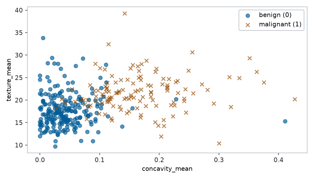
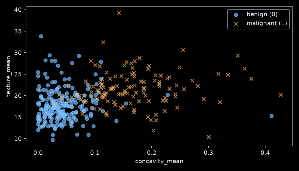
fig, ax = plt.subplots(figsize=(7, 4))for label, name, marker in [(0, "benign (0)", "o"), (1, "malignant (1)", "x")]: group = y == label ax.scatter(X[group, 0], X[group, 1], label=name, marker=marker, alpha=0.65)ax.set(xlabel="concavity_mean", ylabel="texture_mean")ax.legend()fig.tight_layout()show_plot(fig)
Figure 8.1: Training data only: concavity and texture partly separate the two labels. Their scales differ greatly, and their correlation is moderate (about 0.34 in this split).
Predict first — Core, 5 minutes. Sketch a straight boundary. Which mistakes remain? Would “always benign” achieve a nonzero accuracy? Would that make it useful for finding malignant cases?
8.2.2 A probability model to try before deriving it
Keep the affine score from Week 1,
\[
z=b+w_1x_1+w_2x_2,
\]
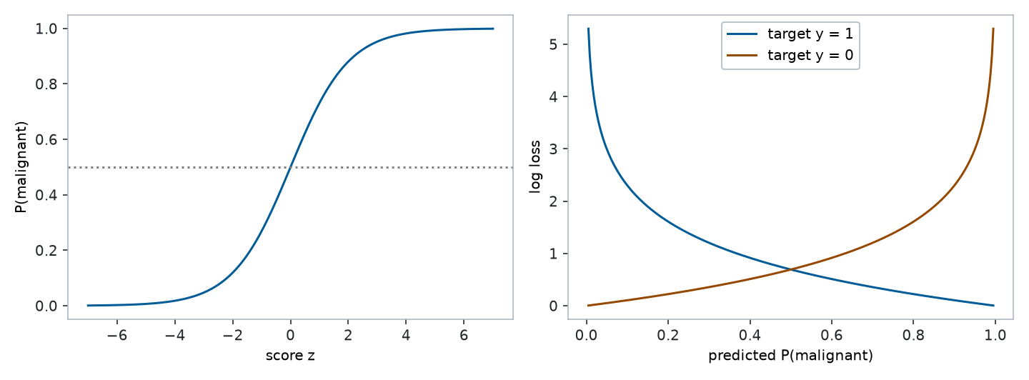
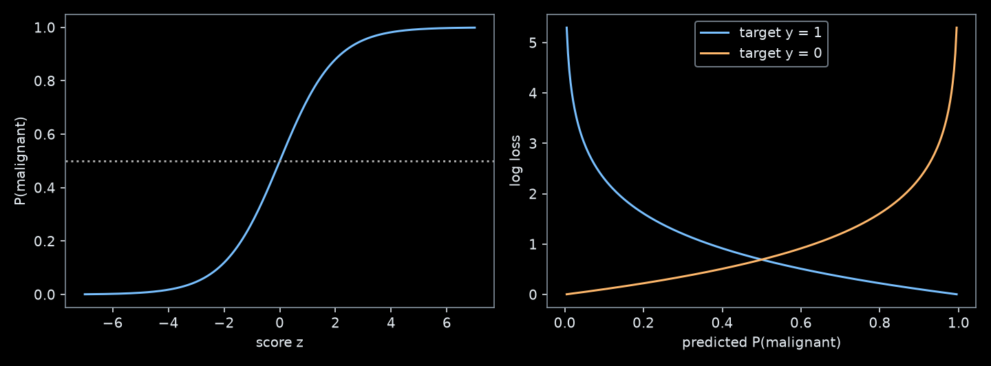
but pass it through the sigmoid\(\sigma(z)=1/(1+e^{-z})\) to obtain a number between zero and one. For now, treat this as a recipe. We will justify it below. A probability of at least \(0.5\) produces label 1; that threshold is a separate choice from the probability model.
The next cell supplies a scoring rule: log loss. Lower is better; a confident wrong prediction is expensive. Its formula and derivative are the next learning goal, not a prerequisite for trying the cell.
def sigmoid(z):# Algebraically 1 / (1 + exp(-z)), evaluated without overflow.return np.exp(-np.logaddexp(0.0, -np.asarray(z)))def design(features):# Rows: examples. Columns: 1, concavity, texture.return np.column_stack((np.ones(len(features)), features))def loss(A, targets, theta): z = A @ thetareturn np.mean(np.logaddexp(0.0, z) - targets * z)A = design(X)A_valid = design(X_valid)# Parameter order is ALWAYS intercept, concavity weight, texture weight.theta_try = np.array([-3.0, 20.0, 0.05]) # Try at most five alternatives.p_try = sigmoid(A @ theta_try)q = y.mean() # Constant baseline estimated on training labels only.baseline_loss =-np.mean(y * np.log(q) + (1- y) * np.log1p(-q))print(f"Your training log loss: {loss(A, y, theta_try):.4f}")print(f"Constant-probability baseline log loss: {baseline_loss:.4f}")print(f"Your accuracy: {np.mean((p_try >=0.5) == y):.3f}")print(f"Always-benign accuracy: {np.mean(y ==0):.3f}")
Your training log loss: 0.3367
Constant-probability baseline log loss: 0.6602
Your accuracy: 0.915
Always-benign accuracy: 0.628
Record the parameter values, loss, and reason for each change. A boundary alone does not show confidence: multiplying all three parameters by ten keeps the \(0.5\) boundary but changes probabilities and log loss. Try this on the training data.
8.2.3 Reuse gradient descent — and encounter slow progress
The following partial derivatives are supplied temporarily. You will derive them shortly. This is full-batch gradient descent with the same zero initialization and a fixed step size in every update. The small step size is chosen from a curvature bound, explained later; it is not selected to make the method fail.
Pause — Core, 5 minutes. The loss decreases, but after 2,000 updates it remains around \(0.629\). Does decreasing loss prove that optimization is nearly finished? What evidence would distinguish an insufficient model from an optimizer that has not yet fitted that model?
Write one prediction about each intervention: more updates, changing feature units, and changing the update rule. We return to the same objective and split after understanding them.
The score\(z\) may be any real number. The probability\(p\) lies between 0 and 1. The decision\(\hat y=\mathbf{1}[p\geq\tau]\) uses a threshold \(\tau\). These are three different quantities. The word regression refers here to modeling a probability through a real-valued score; the observed target is a class label.
Logistic regression assumes that the log odds are affine in the input features. It does not assume that the probability itself is affine. At \(\tau=0.5\), the boundary is \(z=0\). At another threshold it is \(z=\log(\tau/(1-\tau))\): a parallel line, unless both feature weights vanish.
Check it by substituting \(y=0\) and \(y=1\). This is a Bernoulli probability model. Assuming observations are independent conditional on their inputs and the model parameters, multiply their assigned probabilities:
In maximum likelihood estimation (MLE), the inputs and observed labels stay fixed; choose the parameters that make this product largest. It is not a probability distribution over the parameters.
Multiplying many small numbers is inconvenient. The logarithm is increasing, so maximizing the product and maximizing its logarithm have the same solutions. Negate and average to get a minimization objective:
This is binary cross-entropy, also called binary log loss. The factor \(1/n\) changes gradient magnitudes, not the minimizer. Our earlier score is now derived from a probabilistic model.
NoteMath bridge: likelihood on two observations
For labels \((1,0)\) and predicted probabilities \((0.8,0.3)\), the likelihood is \(0.8(1-0.3)=0.56\). For probabilities \((0.6,0.4)\) it is \(0.36\). Both models classify both observations correctly at \(0.5\), but likelihood prefers the first. Accuracy has discarded information about confidence.
Math 3 connection: least squares arose from Gaussian noise in Week 1. Here the Bernoulli model leads to cross-entropy. MLE is the estimation principle; gradient descent and Newton are two algorithms that can carry it out.
8.3.2 Compute the loss from logits, stably
Substitute \(p=\sigma(z)\) and simplify one observation’s loss:
\[
\ell(z,y)=\log(1+e^z)-yz.
\]
Directly computing \(e^z\) can overflow. np.logaddexp(0, z) computes \(\log(e^0+e^z)\) stably. This is why our implementation keeps the logits (the scores) until the loss calculation. PyTorch’s BCEWithLogitsLoss combines sigmoid and the loss in the same spirit; do not apply sigmoid before passing it logits.
These have the same structure as the Week 1 least-squares derivatives: a weighted average of prediction-minus-observation discrepancies. Week 1 writes that discrepancy as \(-r=\hat y-y\), with a factor of 2 for MSE; here it is probability minus binary label, \(p-y\). If \(y=1\) and \(p\) is too small, \(p-y<0\); decreasing the loss requires increasing that example’s score.
For example, at \(\theta=0\), one input \((x_1,x_2)=(0.1,20)\) with \(y=1\) has \(p=0.5\). Its contributions to the three derivatives are \((-0.5,-0.05,-10)\). Equal numerical changes in the two weights do not have equal effects on the score. This is a clue to the scaling problem.
8.4.1 Package the partial derivatives
Let \(\theta=(b,w_1,w_2)^\top\) and let \(A\) contain one row \(\boldsymbol a_i^\top=(1,x_{i1},x_{i2})\) per example. Then
This recovers the supplied function exactly. Gradient descent updates all coordinates from the same current gradient: \(\theta_{t+1}=\theta_t-\eta\boldsymbol g_t\).
# Central differences check the analytic gradient away from initialization.theta_check = np.array([-1.0, 3.0, 0.03])eps =1e-5basis = np.eye(3)g_fd = np.array([ (loss(A, y, theta_check + eps * e) - loss(A, y, theta_check - eps * e)) / (2* eps)for e in basis])np.testing.assert_allclose(gradient(A, y, theta_check), g_fd, rtol=1e-6, atol=1e-7)print("All three partial derivatives agree with finite differences.")
All three partial derivatives agree with finite differences.
Check your understanding. Why would comparing targets with thresholded labels, instead of probabilities, break this derivative? What would happen if y had shape (n, 1) while p had shape (n,)?
8.5 Improve I: change the coordinates
Fit preprocessing on the training set only. Standardize each feature by subtracting its training mean and dividing by its training standard deviation:
\[
\widetilde x_j=\frac{x_j-\mu_j}{s_j}.
\]
With a freely fitted intercept, this changes coordinates but not the set of affine scores the model can represent. In this unregularized experiment it also leaves the attainable minimum loss unchanged. It can change the trajectory of gradient descent substantially.
Standardized GD after 2000 updates: 0.262413
Same feature correlation: 0.341
The loss is now around \(0.262\), much lower than the raw-feature run. The model was capable of a better fit all along. This is an optimization diagnosis, not a generalization result.
ImportantCorrelation and scale are different
These two features are moderately positively correlated: about \(0.30\) across all rows and \(0.34\) in the training split. Their training standard deviations are about \(0.081\) and \(4.31\). Standardization preserves their correlation but greatly improves this run.
Therefore, the severe slowdown here is mainly a scale and centering problem. Correlation can also couple parameter directions and slow gradient descent, especially when predictors are nearly redundant. Correlation alone does not determine convergence; the loss curvature does. The lab creates a deliberately more correlated coordinate system, using only these same two measurements, to isolate that effect.
8.6 Understand: why MLE needs an iterative solution
In the optional Week 1 derivation, setting the least-squares gradient to zero gave linear equations in the parameters. Here stationarity requires
The unknown parameters appear inside a nonlinear sigmoid. In general, binary logistic regression has no closed-form MLE like the least-squares normal-equation solution. Special cases, such as fitting only an intercept, can be solved explicitly. For the general feature-based model, solve the stationarity equations iteratively.
Gradient descent already does this. Can we use more of the local shape to take better steps?
8.6.1 One parameter: use slope and curvature
For a one-dimensional loss \(f(u)\), near the current value \(u\) approximate its slope by
\[
f'(u+d)\approx f'(u)+f''(u)d.
\]
Set the approximate new slope to zero. This gives \(d=-f'(u)/f''(u)\), or the Newton update
\[
u_{\text{new}}=u-\frac{f'(u)}{f''(u)}.
\]
A large second derivative means the slope changes quickly; take a smaller displacement for the same current slope. For a quadratic with positive curvature, this reaches the minimum in one step. Logistic loss is not quadratic, so its curvature must be recomputed.
8.6.2 Three parameters: a table of second partial derivatives
Differentiate the gradient components again. Write \(a_{ij}\) for entry \(j\) of row \(i\), including the intercept column \(a_{i0}=1\):
The \(3\times3\) matrix \(H\) is the Hessian. Diagonal entries describe curvature along individual parameter axes. Off-diagonal entries describe how changing one parameter changes the slope with respect to another. The mixed partial derivatives you know from Math 2 now become a table.
Let \(R=\operatorname{diag}(p_i(1-p_i))\). In matrix form,
\[
H=\frac1nA^\top R A.
\]
We compute this without constructing the full \(n\times n\) diagonal matrix:
def hessian(A, theta): p = sigmoid(A @ theta)return A.T @ ((p * (1- p))[:, None] * A) /len(A)H_check = hessian(A, theta_check)H_fd = np.column_stack([ (gradient(A, y, theta_check + eps * e) - gradient(A, y, theta_check - eps * e)) / (2* eps)for e in basis])np.testing.assert_allclose(H_check, H_check.T, atol=1e-12)np.testing.assert_allclose(H_check, H_fd, rtol=1e-6, atol=1e-7)print("Second partial derivatives also pass their finite-difference check.")
Second partial derivatives also pass their finite-difference check.
Coding bridge.p * (1-p) has shape (n,). Adding [:, None] gives (n, 1), so multiplication scales each row of A by its curvature weight. Then (3, n) @ (n, 3) produces (3, 3).
\[
\boldsymbol v^\top H\boldsymbol v
=\frac1n\sum_i p_i(1-p_i)(\boldsymbol a_i^\top\boldsymbol v)^2\geq0.
\]
Thus the objective is convex: any finite stationary point is a global minimum. If \(A\) has full column rank, the Hessian is positive definite at finite parameters in exact arithmetic. This does not ensure that a finite MLE exists for every dataset; perfectly separable data are an important exception.
A narrow loss valley has large curvature in one direction and small curvature in another. A single learning rate must be cautious in the steep direction, and then may make little progress in the shallow direction. Correlated predictors can tilt and stretch the valley; mismatched feature units can stretch it too.
Depth choice: quantify the shape. The eigenvalues of a positive-definite Hessian measure its curvature along principal directions. Their largest-to-smallest ratio is the condition number. Larger ratios mean more unequal curvature in the chosen coordinates. You do not need to compute eigenvectors by hand for the experiment.
for name, matrix in [("raw", A), ("standardized", B)]: H0 = hessian(matrix, np.zeros(3))print(f"{name:12s}: initial Hessian condition number = {np.linalg.cond(H0):.1f}")
raw         : initial Hessian condition number = 68130.6
standardized: initial Hessian condition number = 2.0
The initial ratios are about \(68{,}131\) and \(2.03\). The ratios change as the fit changes because \(R\) depends on the probabilities. Pearson feature correlation alone is not the weighted curvature at later iterations.
Our gradient-descent step size was not arbitrary: \(0<p_i(1-p_i)\leq1/4\), so curvature is bounded by \(A^\top A/(4n)\). Its largest eigenvalue is a global upper bound \(L\) on the gradient’s rate of change. A step \(\eta=1/L\) is a conservative, stable full-batch choice for this objective. Each coordinate system uses the same rule, rather than the same numerical learning rate with different units.
8.6.4 Newton’s update: solve a small linear system
The multi-parameter slope approximation is
\[
\nabla J(\theta+\boldsymbol d)\approx\boldsymbol g+H\boldsymbol d.
\]
Set it to zero. Equivalently, solve \(H\boldsymbol s=\boldsymbol g\) and update
\[
\theta_{\text{new}}=\theta-\alpha\boldsymbol s.
\]
This is a second-order method because it uses second derivatives. It accounts for coupling between coordinates as well as their separate scales. Solve the linear system; do not explicitly compute \(H^{-1}\).
A full step has \(\alpha=1\). Far from the minimum, a local approximation can be inaccurate. Our damped Newton method halves \(\alpha\) until the actual loss decreases sufficiently (Armijo backtracking). This changes the step, not the statistical objective. No regularization is added to make the comparison work.
def newton(A, targets, max_steps=30, tol=1e-10): theta = np.zeros(A.shape[1]) history = [loss(A, targets, theta)] step_sizes = []for _ inrange(max_steps): g = gradient(A, targets, theta) direction = np.linalg.solve(hessian(A, theta), g) decrement_squared =float(g @ direction)# Predicted improvement of the local quadratic model.if decrement_squared /2<= tol:return theta, np.array(history), np.array(step_sizes) step =1.0while loss(A, targets, theta - step * direction) > history[-1] -1e-4* step * decrement_squared: step *=0.5if step <2**-40:raiseRuntimeError("Line search failed; inspect curvature and data.") theta -= step * direction history.append(loss(A, targets, theta)) step_sizes.append(step)raiseRuntimeError("Newton did not converge within the update budget.")
The stopping quantity \(\boldsymbol g^\top H^{-1}\boldsymbol g/2\) is the predicted decrease of the local quadratic model. It is a local diagnostic, not an exact global error bound. In the following comparison we also use the same loss-gap target for every trajectory.
8.7 Improve II: compare the same fit fairly
Keep the data, labels, split, unpenalized objective, and initial predictions \(p_i=0.5\) fixed. Compare raw and standardized gradient descent with raw and standardized Newton. Here changing coordinates preserves the model family and the initial predictions.
theta_newton_raw, history_newton_raw, steps_raw = newton(A, y)theta_newton, history_newton, steps_scaled = newton(B, y)reference_loss = loss(B, y, theta_newton)np.testing.assert_allclose(A @ theta_newton_raw, B @ theta_newton, atol=1e-8)np.testing.assert_allclose(history_newton_raw, history_newton, atol=1e-12)assert np.linalg.norm(gradient(B, y, theta_newton), ord=np.inf) <1e-8runs = {"GD, raw": history_raw,"GD, standardized": history_scaled,"Newton, raw": history_newton_raw,"Newton, standardized": history_newton,}print("Reference training loss:", round(reference_loss, 6))for name, history in runs.items(): reached = np.flatnonzero(history - reference_loss <=1e-6) first =str(reached[0]) iflen(reached) else"not reached"print(f"{name:22s} loss={history[-1]:.6f}; first update within 1e-6: {first}")print("Newton accepted step sizes:", steps_scaled)
Reference training loss: 0.262413
GD, raw                loss=0.628918; first update within 1e-6: not reached
GD, standardized       loss=0.262413; first update within 1e-6: 80
Newton, raw            loss=0.262413; first update within 1e-6: 5
Newton, standardized   loss=0.262413; first update within 1e-6: 5
Newton accepted step sizes: [1. 1. 1. 1. 1. 1.]
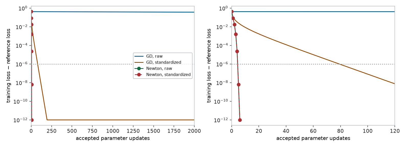
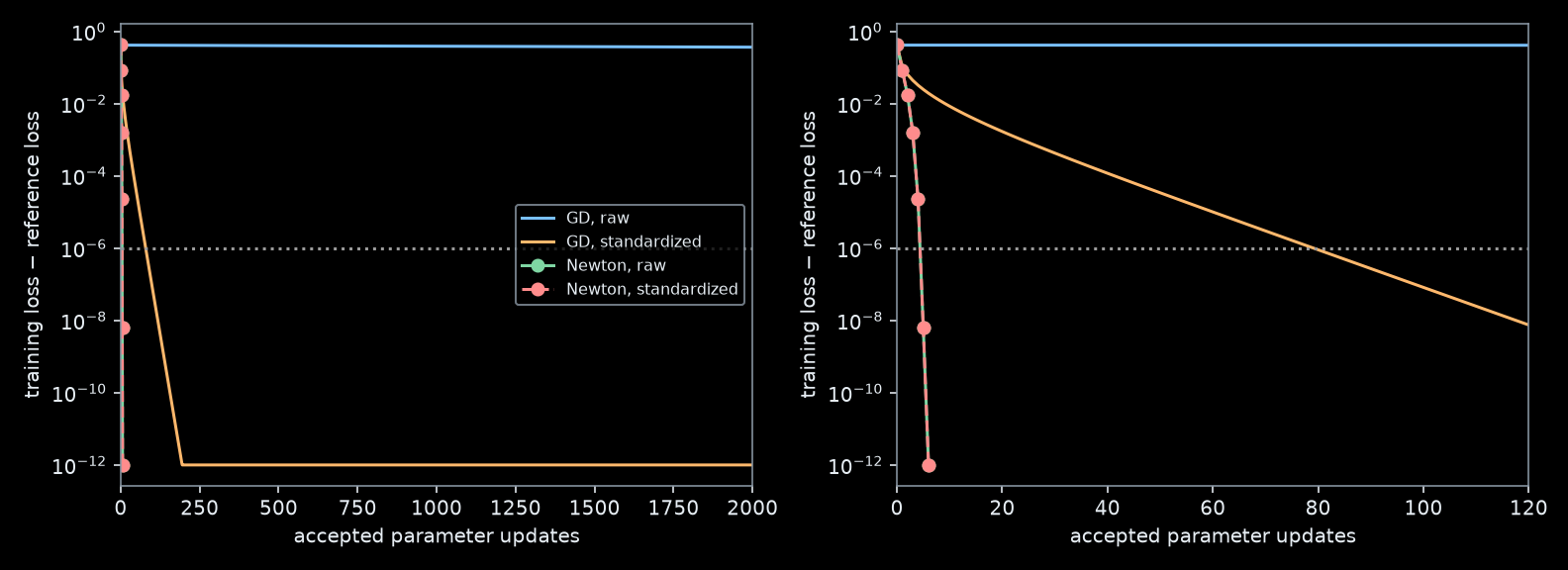
fig, axes = plt.subplots(1, 2, figsize=(11, 4))for ax in axes:for name, history in runs.items(): ax.semilogy(np.maximum(history - reference_loss, 1e-12), label=name, linestyle="--"if name =="Newton, standardized"else"-", marker="o"if name.startswith("Newton") elseNone) ax.axhline(1e-6, color="0.6", linestyle=":") ax.set(xlabel="accepted parameter updates", ylabel="training loss − reference loss")axes[0].set_xlim(0, 2000)axes[1].set_xlim(0, 120)axes[0].legend(fontsize=8)fig.tight_layout()show_plot(fig)
Figure 8.3: Same training objective and initial predictions. Standardization repairs much of GD’s slowdown; Newton reaches the same optimum in six updates in either coordinate system. The right panel zooms into the first 120 updates. Gaps below 1e-12 are clipped only for plotting.
For this split, standardized GD reaches the \(10^{-6}\) loss-gap target at about update 80; Newton reaches it at update 5 and satisfies its stricter internal stopping rule after 6 updates. Raw GD does not reach the target within 2,000 updates. These are reproducible observations under the stated step-size rule, not universal iteration counts.
Interpret the comparison. Newton has not discovered a better model than converged GD. Both minimize the same objective. It gets there in fewer updates by doing more work per update. With \(d\) parameters, a dense Hessian needs \(O(d^2)\) storage and a generic solve costs \(O(d^3)\); constructing it also costs work proportional to the data size. A \(3\times3\) solve is cheap here. This does not establish a wall-clock advantage for large neural networks.
WarningWhen an MLE or Newton step can fail
With complete or certain forms of quasi-complete separation, coefficients can grow without bound while the likelihood approaches a supremum; a finite MLE need not exist. Duplicate feature columns make the Hessian singular. Very confident predictions can make its numerical curvature tiny. Convexity alone fixes none of these issues.
The routine above deliberately reports a failed solve or convergence failure instead of silently changing the objective. Check rank, separation, scaling, and precision. An L2 penalty can stabilize fitting but changes MLE to a penalized objective; the lab studies that as a separate experiment. Backtracking protects the local step and does not create a finite MLE when none exists.
8.8 Return to predictions: fitting is not evaluation
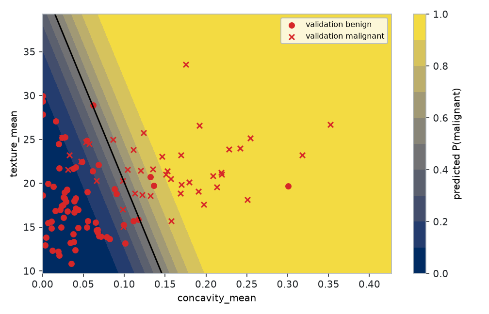
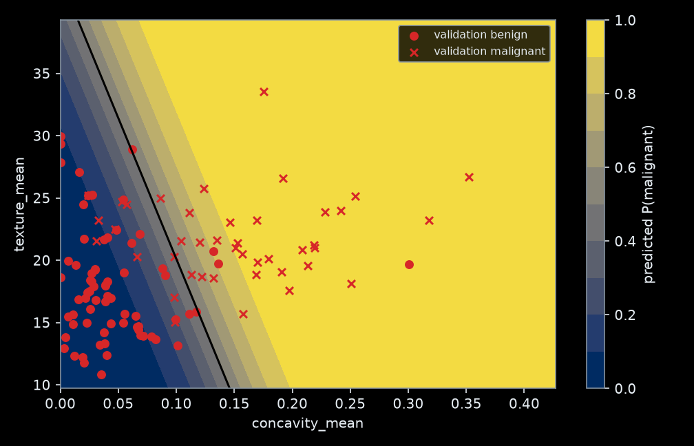
We can now inspect validation probabilities and a boundary without changing the fit. Keep the test set for the final lab checkpoint.
Figure 8.4: The converged two-feature logistic model on a grid, with validation observations and its probability-0.5 boundary. The boundary is straight even though probabilities are nonlinear in the score.
Different questions require different measurements:
Question
Measurement
What it does not establish
Does the model rank malignant examples above benign examples?
AUROC
Calibration or performance at a chosen threshold
Are assigned probabilities useful?
Held-out log loss; Brier score
A complete description of calibration
Are predicted probabilities consistent with observed frequencies?
Reliability plot with bin counts
Reliable clinical calibration from a small sample
What mistakes occur at our threshold?
Confusion matrix, sensitivity, specificity
Threshold-independent ranking quality
The lab implements these checks. For example, sensitivity is the fraction of malignant examples labeled positive; specificity is the fraction of benign examples labeled negative. Lowering a threshold tends to increase sensitivity and decrease specificity. A threshold should reflect the task and be chosen without the test labels.
8.9 From this chapter to neural networks
The components are now separate:
Component
This experiment
Architecture
Affine score followed by a sigmoid
Objective
Mean negative Bernoulli log likelihood
Data pipeline
Fixed stratified split; training-only scaling
Optimizer
Full-batch GD or damped Newton
Evaluation
Held-out probabilities, ranking, and thresholded errors
Recall basis functions from Week 1. Replacing \(\boldsymbol x\) by fixed features \(\boldsymbol\phi(\boldsymbol x)\) gives \(p=\sigma(b+\boldsymbol w^\top\boldsymbol\phi(\boldsymbol x))\). The boundary can then be curved in the original input space, while fitting the final weights remains convex logistic regression. A neural network learns the feature map as well. The Bernoulli loss still applies to a binary output, but joint fitting of hidden layers generally loses this chapter’s convexity.
8.10 Knowledge check and next experiment
Two classifiers make identical decisions. Must they have the same likelihood? Give a two-observation example.
Derive \(\partial J/\partial w_1\) without matrix notation. Where does the factor \(p-y\) come from?
Why is the equation \(A^\top(\sigma(A\theta)-y)=0\) not the least-squares normal equation?
What new information does a Hessian add beyond a gradient?
Why does standardization help here while leaving Pearson correlation unchanged?
Does six Newton updates versus eighty GD updates prove Newton is always faster? Identify the missing cost information.
Does a lower training loss imply better validation performance?
Return to your initial predictions and revise them using evidence. Then complete the lab: verify the derivatives with PyTorch, isolate correlation, and assess predictions. The optional additional material derives the Newton/IRLS connection and explains why “iterative least squares” is still maximum likelihood for logistic regression.
Wolberg, William, Olvi Mangasarian, Nick Street, and W. Street. 1993. Breast Cancer Wisconsin (Diagnostic). UCI Machine Learning Repository. https://doi.org/10.24432/C5DW2B.