From Newton’s method to iteratively reweighted least squares
NoteOptional depth after the common experiment
The main chapter derives Bernoulli likelihood, the gradient, and Newton’s method. This page connects the new method to the least-squares solution from Week 1. It assumes you can read a matrix product and solve a small linear system. Work through the scalar interpretation even if the matrix derivation is new.
Try → understand → improve: try one ordinary least-squares fit to binary labels; identify what it does not model; derive a sequence of weighted least-squares problems that does optimize logistic likelihood.
10.1 Try: apply the Week 1 solution directly
Use exactly the chapter’s two features and training split. The scalar targets are zeros and ones. Least squares can fit these numbers, but an affine output is not constrained to be a probability.
Predict. Would clipping the outputs to \([0,1]\) turn this estimate into the logistic MLE? Would applying a sigmoid after fitting least squares solve the logistic stationarity equation? Neither transformation changes the objective that was optimized. Test the latter prediction:
print("Logistic gradient at the least-squares coefficients:", gradient(A, y, theta_ls))theta_mle, mle_history, _ = newton(A, y)print("Logistic loss at LS coefficients:", loss(A, y, theta_ls))print("Logistic loss at MLE:", loss(A, y, theta_mle))
Logistic gradient at the least-squares coefficients: [ 0.21596935 -0.27471109 -0.15596082]
Logistic loss at LS coefficients: 0.6403967294105761
Logistic loss at MLE: 0.262413276051727
Ordinary least squares on binary responses is sometimes called a linear probability model. It can be studied on its own terms; it is not logistic maximum likelihood.
10.2 Understand: derive an iteratively reweighted problem
We have not assumed Gaussian binary observations. This weighted quadratic is a local approximation used to optimize the Bernoulli objective. Its responses and weights depend on the current parameters, so they must be recomputed after each step. This is iteratively reweighted least squares (IRLS). For logistic regression, a full IRLS update is algebraically the full Newton update.
10.2.1 What is being approximated?
For one example, expand its negative log likelihood locally around the current score \(z_t\):
The working response \(u_t\) lies on the score/log-odds scale; it is not a new label or a probability. It may be negative or greater than one. Its weight \(r\) comes from likelihood curvature, not from a claim that some patients matter less.
Math bridge. At initialization \(z=0\), all \(p=1/2\), all \(r=1/4\), and \(u=4y-2\). The first IRLS step is therefore ordinary least squares on responses \(-2\) and \(2\), with identical weights. After that step, probabilities differ and the weights change. This explains why one least-squares solve is not the logistic MLE.
10.3 Improve: verify the same step by two routes
Use square roots of weights to solve the least-squares system. Forming normal equations can square the condition number; lstsq on the weighted design is preferable to explicitly inverting \(A^\top R A\).
theta_current = np.array([-0.2, 0.5, 0.1])z = A @ theta_currentp = sigmoid(z)r = p * (1- p)assert r.min() >1e-6# This demonstration is deliberately away from saturation.working_response = z + (y - p) / rsqrt_r = np.sqrt(r)theta_irls = np.linalg.lstsq(sqrt_r[:, None] * A, sqrt_r * working_response, rcond=None)[0]theta_newton = theta_current - np.linalg.solve(hessian(A, theta_current), gradient(A, y, theta_current))np.testing.assert_allclose(theta_irls, theta_newton, atol=1e-12)print("Maximum coordinate difference:", np.max(np.abs(theta_irls - theta_newton)))print("Loss before / after one full step:", loss(A, y, theta_current), loss(A, y, theta_irls))
Maximum coordinate difference: 1.7763568394002505e-15
Loss before / after one full step: 0.5108228911207965 0.324071585561428
This verifies one full step. If backtracking selects \(\alpha<1\), use \(\theta_t+\alpha(\theta_{\mathrm{IRLS}}-\theta_t)\) and check the actual logistic loss. Replacing the whole fit by one weighted solve, or keeping the first iteration’s weights forever, changes the algorithm.
When \(p\) is numerically close to zero or one, the working response divides by tiny numbers. The main chapter’s gradient/Hessian implementation avoids explicitly forming that response, though its linear system can still become ill-conditioned. Scaling, stable logits, rank checks, and damping remain useful.
10.4 Why Newton’s trajectory survives a change of coordinates
The chapter found identical loss trajectories for raw and standardized Newton fits. This is more than an accident of one random seed.
Represent an invertible affine change of features, including the intercept, by a nonsingular matrix \(T\) such that \(A_{\mathrm{new}}=AT\). The same score is obtained with \(\theta=T\beta\). By the chain rule,
\[
\boldsymbol g_\beta=T^\top\boldsymbol g_\theta,\qquad
H_\beta=T^\top H_\theta T.
\]
If \(H_\beta\boldsymbol s_\beta=\boldsymbol g_\beta\), multiply through to see that \(T\boldsymbol s_\beta=\boldsymbol s_\theta\). A full Newton update therefore produces the same scores in either coordinate system. The decrement and Armijo condition are also unchanged if initial scores and damping rules match. Finite-precision arithmetic and nearly singular transformations can spoil that agreement.
Plain GD generally does not have this invariance: mapping its step back multiplies the gradient by \(TT^\top\). This is why changing feature units can change a GD trajectory even when the model family stays the same.
10.5 Why a finite solution is not guaranteed
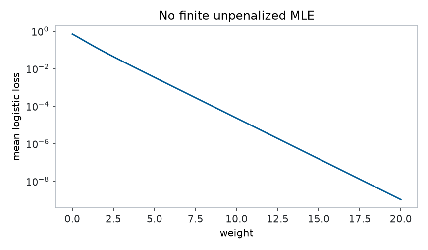
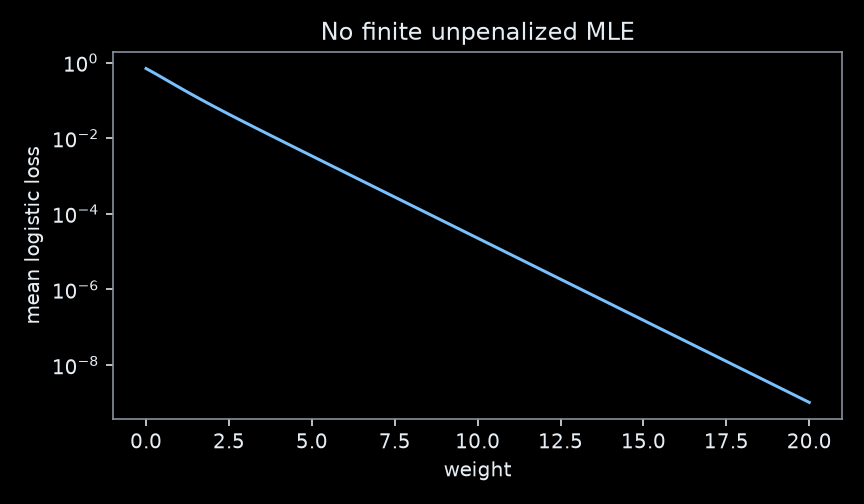
Here is a separate synthetic, perfectly separable example. The intercept is zero and the one feature’s sign exactly determines the label. Increase a positive weight and inspect the loss.
x_separable = np.array([-2.0, -1.0, 1.0, 2.0])y_separable = np.array([0.0, 0.0, 1.0, 1.0])weights = np.linspace(0, 20, 120)# For every example here, its correctly signed margin is w * abs(x).# This form avoids cancellation for large positive, correct scores.separable_losses = np.array([np.logaddexp(0.0, -w * np.abs(x_separable)).mean() for w in weights])fig, ax = plt.subplots(figsize=(6, 3.5))ax.semilogy(weights, separable_losses)ax.set(xlabel="weight", ylabel="mean logistic loss", title="No finite unpenalized MLE")fig.tight_layout()show_plot(fig)
Figure 10.1: A separate, perfectly separable toy dataset: increasing the weight drives logistic loss toward zero without attaining it at any finite weight. This is not the overlapping two-feature WDBC training problem.
For any finite positive weight, every assigned probability is still short of perfect certainty, so the loss remains positive. Larger weights always improve it. A report that Newton “converged” merely because an improvement fell below a tolerance does not prove a finite MLE exists.
An L2 penalty changes the problem and can prevent this divergence. For the small two-feature, overlapping training example used in the chapter, the finite fitted parameters have a tiny gradient and a positive-definite Hessian. Do not transfer that observation to all 30 UCI features or to every classification dataset.
10.6 Check your understanding
At zero initialization, derive the working responses for \(y=0\) and \(y=1\).
Which objects must be recomputed after every IRLS step, and why?
Why can we solve each weighted subproblem in closed form while logistic MLE has no general closed-form solution?
Does a curvature weight near zero mean the example can safely be discarded? Consider a confidently wrong prediction and its working response.
What is preserved under an invertible feature transformation: the coefficients, the representable logits, or both?
Give one reason a Hessian might be numerically singular even when the data matrix has full column rank.
Return to the lab and use one of these results to explain your optimizer comparison.