6 Lab 1: Try, diagnose, improve

From a hand-fitted line to a tested learning procedure

6.1 Workflow and deliverable

Begin after the concepts notebook. This lab runs independently from a fresh kernel; it does not need variables from that page. Work in pairs, switch driver and navigator halfway through, and write your interpretation individually. Start in Session 2; allow 3–4 hours after class, including the core exercises.

Common core: W01-01 through W01-04. Submit an executable regressor, an experiment figure, and a short account of a failed attempt and its repair. Depth choice: one mathematical or coding extension. Enrichment: additional seed or extrapolation studies.

The worked code is complete so that the notebook always executes. The exercises require you to change it, predict an outcome, and explain evidence. Do not treat running every cell as completing the lab.

6.2 Try: transfer your first fitting strategy

A sensor’s calibration now also depends on a second measured feature. The names below are generic because the dataset is synthetic. Use the training measurements to fit the targets; the visible generating coefficients are for reproducibility, not a fitting shortcut.

import matplotlib.pyplot as plt
from dlbook.plotting import show_plot
import torch

DTYPE = torch.float64
rng = torch.Generator().manual_seed(19)
X_all = torch.randn((160, 2), generator=rng, dtype=DTYPE)
y_all = X_all @ torch.tensor([[1.8], [-0.7]], dtype=DTYPE) + 0.4
noise = 0.25 * torch.randn((160, 1), generator=rng, dtype=DTYPE)
y_all = y_all + noise
order = torch.randperm(160, generator=rng)
train, valid, test = order[:100], order[100:130], order[130:]
X, y = X_all[train], y_all[train]
X_valid, y_valid = X_all[valid], y_all[valid]
X_test, y_test = X_all[test], y_all[test]
assert X.shape == (100, 2) and y.shape == (100, 1)

Core, 5 minutes. Try three choices for two weights and a bias. Predict the effect of each change first. Which difficulty from the one-feature experiment persists?

weights_try = torch.tensor([[0.0], [0.0]], dtype=DTYPE)
bias_try = torch.tensor(0.0, dtype=DTYPE)
prediction_try = X @ weights_try + bias_try
print("Training MSE:", ((y - prediction_try) ** 2).mean().item())
print("Feature-free training baseline:", ((y.mean() - y) ** 2).mean().item())

Training MSE: 3.7770957642362704
Feature-free training baseline: 3.555262373956899

6.3 Understand: check what the code is actually computing

For \(n\) examples and \(d\) features, X has shape (n, d) and the weights have shape (d, 1). The product X @ weights has shape (n, 1), matching the target column. Adding a scalar bias shifts each prediction.

6.3.1 A silent failure you can inspect safely

An executable demonstration may show incorrect behavior without crashing the notebook. Here the only change is flattening the targets. Before running, predict the resulting residual shape.

correct_residual = y - prediction_try
wrong_residual = y[:, 0] - prediction_try
print("Correct residual shape:", tuple(correct_residual.shape))
print("Wrong residual shape:  ", tuple(wrong_residual.shape))
assert correct_residual.shape == (100, 1)
assert wrong_residual.shape == (100, 100)

# Unequal predictions expose the semantic error even more clearly.
p_demo = torch.tensor([[1.0], [3.0]], dtype=DTYPE)
y_demo = torch.tensor([[1.0], [3.0]], dtype=DTYPE)
print("Matched-example MSE:", ((y_demo - p_demo) ** 2).mean().item())
print("All-pairs MSE:      ", ((y_demo[:, 0] - p_demo) ** 2).mean().item())

Correct residual shape: (100, 1)
Wrong residual shape:   (100, 100)
Matched-example MSE: 0.0
All-pairs MSE:       2.0

PyTorch expands the (n, 1) prediction down columns and the (n,) target across rows. The wrong expression compares every prediction with every target, rather than matching observations. It still produces a finite mean. Correct-looking output is not sufficient evidence that the intended objective was implemented.

6.3.2 Write and verify the objective and gradient

The gradient contains one derivative for each weight, plus one for the bias. Computing both from the same residual ensures that they refer to the same current parameters.

def predict(features, weights, bias):
    assert features.ndim == 2
    assert weights.shape == (features.shape[1], 1)
    assert bias.ndim == 0
    return features @ weights + bias


def objective(features, targets, weights, bias):
    prediction = predict(features, weights, bias)
    assert prediction.shape == targets.shape
    return (targets - prediction).square().mean()


def derivatives(features, targets, weights, bias):
    residual = targets - predict(features, weights, bias)
    assert residual.shape == targets.shape == (len(features), 1)
    dw = -2 * features.T @ residual / len(features)
    db = -2 * residual.mean()
    return dw, db


w_check = torch.tensor([[0.2], [-0.1]], dtype=DTYPE, requires_grad=True)
b_check = torch.tensor(-0.3, dtype=DTYPE, requires_grad=True)
loss = objective(X, y, w_check, b_check)
loss.backward()
dw, db = derivatives(X, y, w_check.detach(), b_check.detach())
torch.testing.assert_close(dw, w_check.grad)
torch.testing.assert_close(db, b_check.grad)
assert dw.shape == (2, 1) and db.ndim == 0
print("Manual and automatic derivatives agree.")

Manual and automatic derivatives agree.

This comparison checks the derivatives, while the shape checks protect the objective. Neither alone would establish the entire learning system’s correctness.

6.4 Improve: a training loop with visible state

We now reuse the gradient we have just implemented. The history contains loss at the starting point and after each update. A safety stop prevents an unstable experiment from overflowing. A completed budget is not automatically evidence of convergence.

def fit(features, targets, rate=0.1, steps=100):
    weights = torch.zeros((features.shape[1], 1), dtype=features.dtype)
    bias = torch.tensor(0.0, dtype=features.dtype)
    losses = [objective(features, targets, weights, bias).item()]
    for _ in range(steps):
        dw, db = derivatives(features, targets, weights, bias)
        assert torch.isfinite(dw).all() and torch.isfinite(db)
        weights = weights - rate * dw
        bias = bias - rate * db
        losses.append(objective(features, targets, weights, bias).item())
        if not torch.isfinite(torch.tensor(losses[-1])) or losses[-1] > 1e12:
            return weights, bias, losses, "stopped: unstable"
    return weights, bias, losses, "budget completed"


weights, bias, losses, status = fit(X, y)
assert losses[-1] < losses[0]
# An independent solver checks the fitted result, not just that loss decreased.
design = torch.cat((X, torch.ones((len(X), 1), dtype=DTYPE)), dim=1)
reference = torch.linalg.lstsq(design, y).solution
torch.testing.assert_close(weights, reference[:-1], atol=1e-6, rtol=1e-6)
torch.testing.assert_close(bias, reference[-1, 0], atol=1e-6, rtol=1e-6)
print("Weights:", weights[:, 0].tolist(), "bias:", bias.item(), status)

Weights: [1.7921998132955734, -0.7202634527244625] bias: 0.3768414512196406 budget completed

6.5 Controlled experiment

6.5.1 First comparison: learning rate

Hypothesis: too large a learning rate increases the objective despite a correct gradient. Change only the rate; keep the dataset, split, zero initialization, full-batch gradients, and maximum of 100 updates fixed. Predeclare rates 0.005, 0.1, and 1.2.

Three log-scale loss curves contrast slow learning, stable convergence, and an unstable large learning rate. — Figure 6.1: Training MSE at a fixed maximum update budget, changing only the learning rate. Safety-stopped runs retain their failure history.

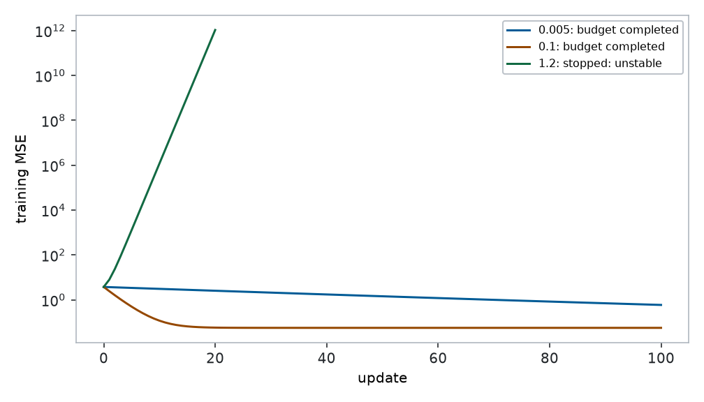
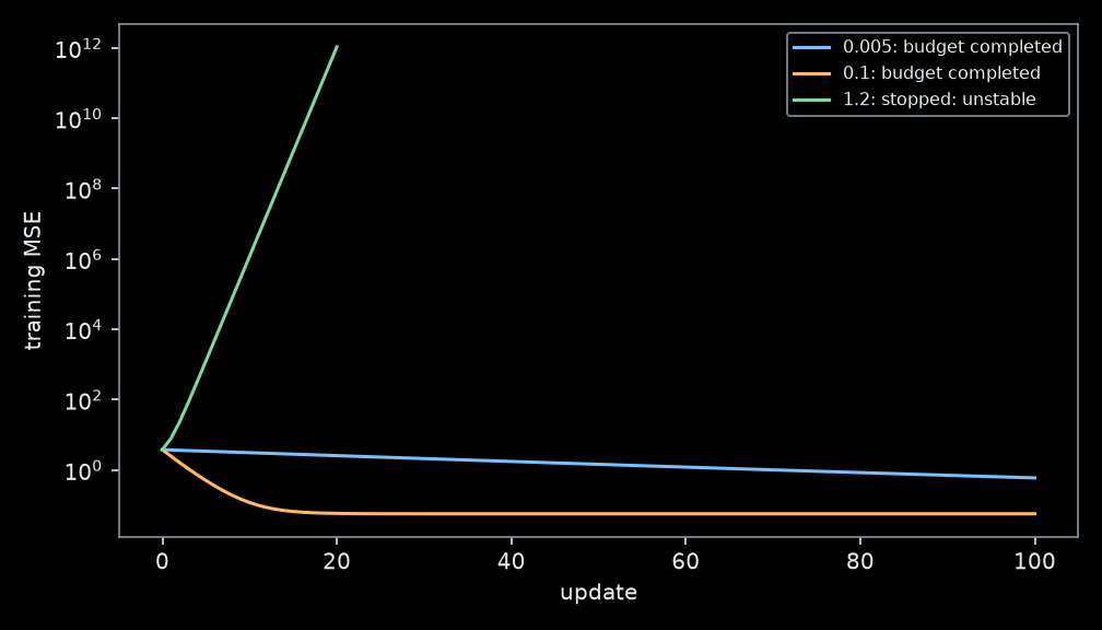
Core checkpoint: report the failed run as a result. Explain the repair using the local approximation from the concepts notebook. A curve that falls slowly requires a different diagnosis from one that rises.

6.5.2 Second comparison: change units, then repair the geometry

Suppose the second sensor reading is now expressed in units one hundred times smaller: its numerical values become one hundred times larger. The targets remain unchanged. No information has been added or removed, and the same affine prediction functions are still available by dividing the second coefficient by 100. But gradient descent sees different numerical derivatives.

Prediction: applying rate 0.1 unchanged to these raw features will fail; standardizing the training features will repair the problem at this budget. Change only preprocessing in the two experimental arms. Use the same training rows, targets, zero predictions at initialization, learning rate, and update limit. This compares optimization under these settings, not every possible optimizer or rate.

unit_scale = torch.tensor([1.0, 100.0], dtype=DTYPE)
X_raw = X * unit_scale
X_valid_raw = X_valid * unit_scale
X_test_raw = X_test * unit_scale

# Fit preprocessing on the training split only.
mean = X_raw.mean(dim=0)
std = X_raw.std(dim=0, unbiased=False)
assert (std > 0).all()  # Constant features need separate handling.
X_scaled = (X_raw - mean) / std
X_valid_scaled = (X_valid_raw - mean) / std
X_test_scaled = (X_test_raw - mean) / std

raw_fit = fit(X_raw, y, rate=0.1, steps=100)
scaled_fit = fit(X_scaled, y, rate=0.1, steps=100)
print("Raw:   ", raw_fit[3], "MSE:", raw_fit[2][-1])
print("Scaled:", scaled_fit[3], "MSE:", scaled_fit[2][-1])
assert raw_fit[3] == "stopped: unstable"
assert scaled_fit[3] == "budget completed"

Raw:    stopped: unstable MSE: 29162328304176.094
Scaled: budget completed MSE: 0.056814060395785126

Raw ill-scaled features produce an increasing loss curve, while standardized features produce a decreasing curve that reaches a low plateau. — Figure 6.2: Same targets, learning rate, initialization in prediction space, and maximum update budget. Training-only standardization changes the optimization geometry.

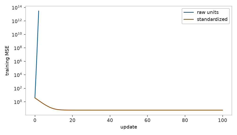
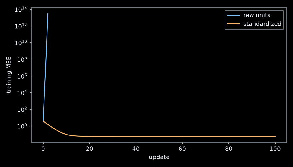
Standardization subtracts each feature’s training mean and divides by its training standard deviation. Equal numerical parameter steps then act on features of more comparable scale. The feature means become zero and standard deviations one in the training data; validation and test values need not have those exact statistics.

We can verify that the model family has not changed. If a standardized fit has weights \(w'_j\) and bias \(b'\), its raw-unit parameters are

\[ w_j=\frac{w'_j}{s_j},\qquad b=b'-\sum_j\frac{w'_j\mu_j}{s_j}, \]

where \(\mu_j\) and \(s_j\) are the training mean and standard deviation of raw feature \(j\).

scaled_weights, scaled_bias = scaled_fit[:2]
raw_equivalent_weights = scaled_weights / std[:, None]
raw_equivalent_bias = scaled_bias - mean @ raw_equivalent_weights[:, 0]
torch.testing.assert_close(
    predict(X_valid_scaled, scaled_weights, scaled_bias),
    predict(X_valid_raw, raw_equivalent_weights, raw_equivalent_bias),
)
print("Changing coordinates preserves predictions on validation examples.")

Changing coordinates preserves predictions on validation examples.

Core checkpoint: which claim did we establish: that standardization expands the model family, or that it helps this optimizer at the stated rate? Would fitting mean and std on all rows respect the split?

6.6 Compare full-batch and minibatch learning

An epoch processes every training example once. Here 100 training rows give one update per epoch at batch size 100 and ten at batch size 10. Compare equal epochs: the nominal number of examples used to calculate updates is equal, but the number of parameter updates is not. We make no speed claim from these curves.

Hypothesis: with the same rate, minibatch learning reaches a similar low-loss region but may fluctuate because successive batches give different gradient estimates. Record full-training MSE at each epoch boundary so the plotted objective is the same in both arms. Both runs use standardized data, zero initialization, 40 epochs, and deterministic shuffling.

def fit_batches(features, targets, batch_size, rate=0.05, epochs=40):
    weights = torch.zeros((features.shape[1], 1), dtype=features.dtype)
    bias = torch.tensor(0.0, dtype=features.dtype)
    generator = torch.Generator().manual_seed(23)
    history = [objective(features, targets, weights, bias).item()]
    for _ in range(epochs):
        permutation = torch.randperm(len(features), generator=generator)
        for start in range(0, len(features), batch_size):
            indices = permutation[start:start + batch_size]
            dw, db = derivatives(features[indices], targets[indices], weights, bias)
            weights, bias = weights - rate * dw, bias - rate * db
        history.append(objective(features, targets, weights, bias).item())
    assert torch.isfinite(torch.tensor(history)).all()
    return weights, bias, history


batch_runs = {size: fit_batches(X_scaled, y, size) for size in (100, 10)}

Loss curves for batch sizes 100 and 10 against epochs. Both approach a low-loss region; the smaller batch uses more updates per epoch. — Figure 6.3: Full-training MSE at epoch boundaries. Equal epochs mean equal passes through the data, with different numbers of updates.

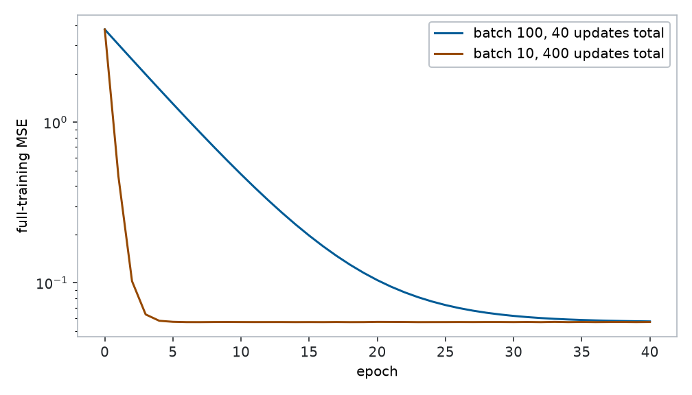
Do not conclude that one batch size is universally better from this one dataset and learning rate. Smaller-batch curves can fluctuate; this is a possibility, not a requirement at every epoch boundary.

6.7 Connect the transparent loop to PyTorch

nn.Linear(2, 1) implements our affine model. Its stored weight shape is (1, 2), so PyTorch transposes it internally. SGD subtracts the learning rate times the stored derivatives; with the full dataset passed below, this optimizer performs full-batch gradient descent despite its name.

The following is a worked reference, after the manual mechanism has been taught. Zero initialization is intentional for this convex model; it is not a general recommendation for hidden layers in neural networks.

model = torch.nn.Linear(2, 1, dtype=DTYPE)
with torch.no_grad():
    model.weight.zero_()
    model.bias.zero_()
optimizer = torch.optim.SGD(model.parameters(), lr=0.1)
for _ in range(100):
    optimizer.zero_grad()       # Clear old derivatives.
    prediction = model(X_scaled)
    assert prediction.shape == y.shape
    loss = (y - prediction).square().mean()
    loss.backward()             # Compute derivatives, without changing parameters.
    optimizer.step()            # Update parameters using those derivatives.

torch.testing.assert_close(model.weight.detach().T, scaled_weights, atol=1e-10, rtol=1e-10)
torch.testing.assert_close(model.bias.detach()[0], scaled_bias, atol=1e-10, rtol=1e-10)
print("Framework and manual full-batch parameters agree.")

Framework and manual full-batch parameters agree.

6.8 Finish the experiment before opening the test results

Use training curves to diagnose optimization, and validation data to assess your model choices. For the worked example, select the standardized full-batch model with rate 0.1 and 100 updates. Confirm the validation result below; freeze the choice before running the test cell. If your experiments motivate another choice, record it first.

validation_mse = objective(X_valid_scaled, y_valid, scaled_weights, scaled_bias).item()
print(f"Selected model validation MSE: {validation_mse:.4f}")

Selected model validation MSE: 0.0711

This final report compares the selected model with the training-mean baseline. It is not a new hyperparameter-selection step.

with torch.no_grad():
    final_prediction = model(X_test_scaled)
    final_rmse = (y_test - final_prediction).square().mean().sqrt().item()
    baseline_rmse = (y.mean() - y_test).square().mean().sqrt().item()
print(f"Test RMSE: model={final_rmse:.4f}; training-mean baseline={baseline_rmse:.4f}")
assert final_rmse < baseline_rmse

Test RMSE: model=0.3031; training-mean baseline=1.7966

6.9 Exercises

6.9.1 Core

Predict, try, explain. On the concepts dataset, record three manual guesses. Explain one proposed change using the sign of a partial derivative, then compare your best guess with gradient descent. A good first guess is allowed; explain what automation adds.
One update by hand. Use \(x=(1,2)\), \(y=(2,3)\) and \(w=1,b=0\). Compute predictions, residuals, MSE, the gradient, and the result after one update at rate 0.1. Check your work with code.
Repair an unsuccessful run. Choose the learning-rate or scaling experiment. State the controls, hypothesis, failed result, one repair, and observed outcome. Include the failure curve rather than hiding it.
Budget matters. Explain how many updates the two minibatch experiments used, and why equal epochs and equal updates are different comparisons. Propose an equal-update comparison without claiming both budgets can be held equal.
Generalization. Identify one optimization claim and one held-out prediction claim your results support. Give one plausible change in measurement conditions they do not cover.

6.9.2 Mathematics bridge

Differentiate \((wx+b-y)^2\) with respect to \(w\) and \(b\) for a single observation. Label the outer and inner derivatives, then average over examples.
Draw the ordered pair of partial derivatives as an arrow. Explain why reversing their order changes the algorithm even though both numbers are correct derivatives.
Show that the training-target mean minimizes the MSE of a constant predictor. This uses one derivative; it does not require maximum likelihood.

6.9.3 Coding bridge

Replace -2 * X.T @ residual / len(X) by loops over examples and features; verify agreement on five rows. State each intermediate shape.
Change the target shape deliberately in a copy of the objective. Demonstrate that your assertion catches the mistake before fitting. Catch the expected exception so the notebook can still run top to bottom.
Add a log entry every tenth update containing the weight values, bias, and MSE. Explain why recording the initial loss separately matters when comparing histories.

6.9.4 Stretch

Math 3 connection. Derive the normal equations or the Gaussian likelihood connection from the concepts page. Identify assumptions; explain why MSE does not itself require Gaussian observations.
Step-size scaling. Repeat the raw-unit experiment with a smaller learning rate and a longer budget. Can you reach the same training fit? Discuss why fixing instability can still leave slow progress in another direction.
Repeated evidence. Repeat the batch comparison across five shuffle seeds while keeping the data split fixed. Distinguish variability from training order from variability due to sampling new data.
Model limitation. Add a quadratic term to a new synthetic target. Fit the affine model, plot residuals against the affected input, and distinguish model mismatch from an optimizer failure. Then use the additional material on basis functions to fit a quadratic feature map and explain what changed. Keep test targets out of feature selection.

6.10 Submission and reflection

Submit your executable notebook, one controlled-comparison figure with both unsuccessful and repaired runs, and a 200–300 word interpretation. Name the changed factor, the fixed quantities, the comparison budget, and one limit of the conclusion. Include the batch-size comparison and an explanation of its budget. Declare substantive collaboration and AI assistance, and be ready to explain one update without an assistant.

Your reflection should complete: “At first I tried …; the theory suggested …; after changing … the evidence showed …; this does not establish ….”

6.11 Summary

The model, objective, gradient, and update retain their meanings when a second feature is added. Shape checks protect the intended computation. A large learning rate and unequal feature scales can defeat otherwise correct updates. A held-out evaluation asks a further question that a low training loss cannot answer.

Return to the concepts notebook for the gradient derivation. Use Python and tensors for shape practice and experiment design for comparisons. Further reading: Zhang et al. (2023), Chapter 3.