Normed spaces#
Norms generalize the notion of length from Euclidean space.
A norm on a real vector space \(V\) is a function \(\|\cdot\| : V \to \mathbb{R}\) that satisfies
(i) \(\|\mathbf{x}\| \geq 0\), with equality if and only if \(\mathbf{x} = \mathbf{0}\)
(ii) \(\|\alpha\mathbf{x}\| = |\alpha|\|\mathbf{x}\|\)
(iii) \(\|\mathbf{x}+\mathbf{y}\| \leq \|\mathbf{x}\| + \|\mathbf{y}\|\) (the triangle inequality again)
for all \(\mathbf{x}, \mathbf{y} \in V\) and all \(\alpha \in \mathbb{R}\).
A vector space endowed with a norm is called a normed vector space, or simply a normed space.
Note that any norm on \(V\) induces a distance metric on \(V\):
\(d(\mathbf{x}, \mathbf{y}) = \|\mathbf{x}-\mathbf{y}\|\)
One can verify that the axioms for metrics are satisfied under this definition and follow directly from the axioms for norms. Therefore any normed space is also a metric space.
We will typically only be concerned with a few specific norms on \(\mathbb{R}^n\):
Here’s a visualization of the unit norm balls in \(\mathbb{R}^2\) for the most common norms:
\(\ell_p\) norms for different values of \(p\) \( p = 1, 2, 3, \infty \)
A counterexample for \( p = 0.5 \), shown as a dashed line, labeled clearly as “not a norm”
These “balls” show the set of all points \(\mathbf{x} \in \mathbb{R}^2\) such that \(\|\mathbf{x}\| = 1\) under each norm.
Show code cell source
import numpy as np
import matplotlib.pyplot as plt

def unit_norm_ball(p, num_points=300):
    """
    Generate points on the unit ball of the Lp norm in R^2.
    """
    theta = np.linspace(0, 2 * np.pi, num_points)
    x = np.cos(theta)
    y = np.sin(theta)

    if p == np.inf:
        # Infinity norm: max(|x|, |y|) = 1 (a square)
        return np.array([
            [-1, -1], [1, -1], [1, 1], [-1, 1], [-1, -1]  # square
        ]).T
    else:
        norm = (np.abs(x)**p + np.abs(y)**p)**(1/p)
        return x / norm, y / norm

# Norm values to plot
norms = [0.5, 1, 2, 3, np.inf]
colors = ['gray', 'red', 'blue', 'green', 'orange']
styles = ['--', '-', '-', '-', '-']
labels = [
    r"$\|\mathbf{x}\|_{0.5}$ (not a norm)",
    r"$\|\mathbf{x}\|_1$",
    r"$\|\mathbf{x}\|_2$",
    r"$\|\mathbf{x}\|_3$",
    r"$\|\mathbf{x}\|_\infty$"
]

# Set up plot
plt.figure(figsize=(8, 8))

for p, color, style, label in zip(norms, colors, styles, labels):
    x, y = unit_norm_ball(p)
    plt.plot(x, y, linestyle=style, color=color, label=label)

# Decorations
plt.gca().set_aspect('equal')
plt.title("Unit Norm Balls in $\\mathbb{R}^2$")
plt.xlabel("$x_1$")
plt.ylabel("$x_2$")
plt.axhline(0, color='black', linewidth=0.5)
plt.axvline(0, color='black', linewidth=0.5)
plt.grid(True, linestyle=':')
plt.legend()
plt.tight_layout()
plt.show()
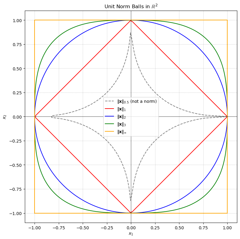
The solid curves for \( p = 1, 2, 3, \infty \) all enclose convex shapes—valid norm balls.
The dashed gray curve for \( p = 0.5 \) appears star-shaped and non-convex, violating the triangle inequality and thus not forming a norm.
It’s a powerful visual cue for why the condition \( p \geq 1 \) is essential for valid norms.
Note that the 1- and 2-norms are special cases of the \(p\)-norm, and the \(\infty\)-norm is the limit of the \(p\)-norm as \(p\) tends to infinity. We require \(p \geq 1\) for the general definition of the \(p\)-norm because the triangle inequality fails to hold if \(p < 1\). (Try to find a counterexample!)
Here’s a fun fact: for any given finite-dimensional vector space \(V\), all norms on \(V\) are equivalent in the sense that for two norms \(\|\cdot\|_A, \|\cdot\|_B\), there exist constants \(\alpha, \beta > 0\) such that
for all \(\mathbf{x} \in V\). Therefore convergence in one norm implies convergence in any other norm. This rule may not apply in infinite-dimensional vector spaces such as function spaces, though.
Normed Spaces in Machine Learning#
Normed spaces generalize the idea of length and thus naturally appear whenever machine learning algorithms quantify vector magnitude or enforce regularization.
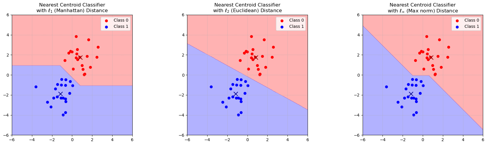
Nearest Centroid Classifier under different norms#
Let’s visualize how different norms affect the decision boundary of a nearest centroid classifier.
Show code cell source
import numpy as np
import matplotlib.pyplot as plt
np.random.seed(42)
# Generate simple 2D synthetic data
class1 = np.random.randn(20, 2) + np.array([1, 2])
class2 = np.random.randn(20, 2) + np.array([-1, -2])
X = np.vstack((class1, class2))
y = np.array([0]*20 + [1]*20)

# Compute centroids
centroids = np.array([X[y==0].mean(axis=0), X[y==1].mean(axis=0)])

# Define metrics
def lp_distance(x, c, p):
    if p == np.inf:
        return np.max(np.abs(x - c), axis=-1)
    else:
        return np.sum(np.abs(x - c) ** p, axis=-1) ** (1/p)

# Grid for plotting decision boundaries
grid_x, grid_y = np.meshgrid(np.linspace(-6, 6, 400), np.linspace(-6, 6, 400))
grid = np.stack((grid_x.ravel(), grid_y.ravel()), axis=1)

# Plot boundaries for each norm
norms = [1, 2, np.inf]
titles = [r"$\ell_1$ (Manhattan)", r"$\ell_2$ (Euclidean)", r"$\ell_\infty$ (Max norm)"]

fig, axs = plt.subplots(1, 3, figsize=(18, 5))

for ax, p, title in zip(axs, norms, titles):
    # Compute distances to each centroid
    d0 = lp_distance(grid, centroids[0], p)
    d1 = lp_distance(grid, centroids[1], p)

    # Predict by choosing the closer centroid
    pred = np.where(d0 < d1, 0, 1)
    pred = pred.reshape(grid_x.shape)

    # Plot decision boundary
    ax.contourf(grid_x, grid_y, pred, levels=1, alpha=0.3, colors=["red", "blue"])

    # Plot data points and centroids
    ax.scatter(class1[:, 0], class1[:, 1], color="red", label="Class 0")
    ax.scatter(class2[:, 0], class2[:, 1], color="blue", label="Class 1")
    ax.scatter(*centroids[0], color="darkred", s=100, marker="x")
    ax.scatter(*centroids[1], color="darkblue", s=100, marker="x")


    ax.set_title(f"Nearest Centroid Classifier\nwith {title} Distance")
    ax.set_xlim(-6, 6)
    ax.set_ylim(-6, 6)
    ax.set_aspect("equal")
    ax.grid(True, linestyle=":")
    ax.legend()

plt.tight_layout()
plt.show()
Regularization#
Regularization methods in machine learning, such as L2 regularization and L1 regularization, explicitly use norms on parameter vectors \(\mathbf{w}\) of models to control overfitting. Regularization adds a penalty term to the loss function, which is often based on the norm of the weights:
General Form:
where \(\Omega(\mathbf{w})\) is a regularization term that penalizes large weights.
By controlling the norm of the weight vector, regularization methods strike a balance between fitting the training data well to achieve a small error and maintaining a level of simplicity that promotes good generalization performance by achieving a small regularizer \(\Omega\). The interplay between the choice of norm for \(\Omega\) and the error term is central to many machine learning applications.
L2 Regularization:
(penalizes the squared Euclidean norm, encouraging small parameter values.)
L1 Regularization (Lasso):
(penalizes the sum of absolute parameter values, promoting sparsity in the solution.)
Regularization in Linear Classification#
In linear classification, regularization controls the complexity of the decision boundary by adding a penalty term to the loss function that is proportional to a norm of the weight vector \(\mathbf{w}\). For example, L₂ regularization (ridge) penalizes \(\|\mathbf{w}\|_2^2\), which encourages the classifier to have smaller weights and hence a smoother decision boundary. In contrast, L₁ regularization (lasso) penalizes \(\|\mathbf{w}\|_1\), promoting sparsity by driving some weight components to zero. This often results in more interpretable models that rely only on the most important features. The decision function
geometrically defines a hyperplane with normal vector \(\mathbf{w}\). The regularization norm affects the magnitude (and, for L₁, the sparsity) of \(\mathbf{w}\), which in turn affects how the hyperplane is placed and how robustly it separates classes.
The geometry of the decision boundary is intimately related to the norm of \(\mathbf{w}\): for example, the distance of a point from the hyperplane is proportional to the projection of \(\mathbf{x}\) onto \(\mathbf{w}\). To enforce simplicity (and avoid overfitting), regularization methods add a penalty based on the norm of \(\mathbf{w}\) to the loss function. Two common regularization strategies in linear classification are:
L₂ Regularization (Ridge):
The regularization term is \(\lambda \|\mathbf{w}\|_2^2\), which penalizes large weights by applying a quadratic penalty. This encourages the classifier to have a small, smoothly distributed weight vector. The resulting decision boundary tends to be smooth and robust to noise.L₁ Regularization (Lasso):
The regularization term is \(\lambda \|\mathbf{w}\|_1\), which penalizes the sum of the absolute values of the weights. This penalty not only discourages large weights but also promotes sparsity, effectively performing feature selection. The decision boundaries from L₁-regularized classifiers often rely on a smaller subset of features, which can lead to more interpretable models.
Show code cell source
import numpy as np
import matplotlib.pyplot as plt
from sklearn.linear_model import LogisticRegression

# Seed for reproducibility.
np.random.seed(42)

# Generate synthetic data for two classes in 2D.
# Class 0 centered at (2, 0.2), Class 1 centered at (-2, -0.2)
n_samples = 20
X_class0 = np.random.randn(n_samples, 2)*1.5 + np.array([2, 0.2])
X_class1 = np.random.randn(n_samples, 2)*1.5 + np.array([-2, -0.2])
X = np.vstack((X_class0, X_class1))
y = np.array([0] * n_samples + [1] * n_samples)

# Fit logistic regression with L2 regularization.
clf_l2 = LogisticRegression(penalty='l2', C=1.0, solver='lbfgs')
clf_l2.fit(X, y)
w_l2 = clf_l2.coef_[0]
b_l2 = clf_l2.intercept_[0]
norm_w_l2 = np.linalg.norm(w_l2)  # L2-norm of the weight vector

# Fit logistic regression with L1 regularization.
clf_l1 = LogisticRegression(penalty='l1', C=1.0, solver='liblinear')
clf_l1.fit(X, y)
w_l1 = clf_l1.coef_[0]
b_l1 = clf_l1.intercept_[0]
norm_w_l1 = np.sum(np.abs(w_l1))  # L1-norm of the weight vector

# Create a meshgrid for plotting decision boundaries.
x_min, x_max = X[:, 0].min() - 1, X[:, 0].max() + 1
y_min, y_max = X[:, 1].min() - 1, X[:, 1].max() + 1
xx, yy = np.meshgrid(np.linspace(x_min, x_max, 400),
                     np.linspace(y_min, y_max, 400))
grid = np.c_[xx.ravel(), yy.ravel()]

# Compute probability predictions for each classifier on the grid.
Z_l2 = clf_l2.predict_proba(grid)[:, 1].reshape(xx.shape)
Z_l1 = clf_l1.predict_proba(grid)[:, 1].reshape(xx.shape)

# Initialize figure with two subplots.
fig, axs = plt.subplots(1, 2, figsize=(14, 6))

# Subplot for L2 regularization.
axs[0].contourf(xx, yy, Z_l2, levels=np.linspace(0, 1, 20), cmap="RdBu", alpha=0.6)
axs[0].contour(xx, yy, Z_l2, levels=[0.5], colors="k")
scatter0 = axs[0].scatter(X[:, 0], X[:, 1], c=y, cmap="RdBu", edgecolor='k')
label_l2 = f"w = [{w_l2[0]:.2f}, {w_l2[1]:.2f}] (||w||₂ = {norm_w_l2:.2f})"
origin_l2 = np.mean(X, axis=0)
axs[0].quiver(origin_l2[0], origin_l2[1], w_l2[0], w_l2[1],
              color='k', scale=5, width=0.005, label=label_l2)
axs[0].set_title("L2 Regularization")
axs[0].set_xlim(x_min, x_max)
axs[0].set_ylim(y_min, y_max)
axs[0].set_xlabel("$x_1$")
axs[0].set_ylabel("$x_2$")
axs[0].grid(True, linestyle=":")
axs[0].legend(loc='upper right')

# Subplot for L1 regularization.
axs[1].contourf(xx, yy, Z_l1, levels=np.linspace(0, 1, 20), cmap="RdBu", alpha=0.6)
axs[1].contour(xx, yy, Z_l1, levels=[0.5], colors="k")
scatter1 = axs[1].scatter(X[:, 0], X[:, 1], c=y, cmap="RdBu", edgecolor='k')
label_l1 = f"w = [{w_l1[0]:.2f}, {w_l1[1]:.2f}] (||w||₁ = {norm_w_l1:.2f})"
origin_l1 = np.mean(X, axis=0)
axs[1].quiver(origin_l1[0], origin_l1[1], w_l1[0], w_l1[1],
              color='k', scale=5, width=0.005, label=label_l1)
axs[1].set_title("L1 Regularization")
axs[1].set_xlim(x_min, x_max)
axs[1].set_ylim(y_min, y_max)
axs[1].set_xlabel("$x_1$")
axs[1].set_ylabel("$x_2$")
axs[1].grid(True, linestyle=":")
axs[1].legend(loc='upper right')

plt.suptitle("Logistic Regression Decision Boundaries\nComparing L2 and L1 Regularization Effects", fontsize=16)
plt.tight_layout(rect=[0, 0.03, 1, 0.95])
plt.show()
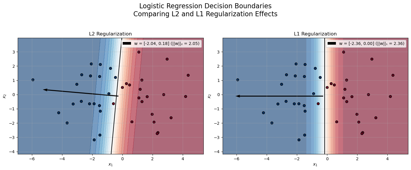
In this visualization, logistic regression is used with two regularization methods: L2 and L1. The weight vector \(\mathbf{w}\) of the classifier is normal to the decision boundary. Its magnitude significantly influences the decision boundary’s placement: L2 Regularization (Ridge) penalizes the squared Euclidean norm \(\|\mathbf{w}\|_2^2\), leading to a dense, smoothly distributed weight vector. The decision boundary is angled according to the balanced contributions of both features. L1 Regularization (Lasso) penalizes the sum of absolute values, \(\|\mathbf{w}\|_1\), which promotes sparsity by driving some components of \(\mathbf{w}\) toward zero. In our example, this results in a vertical decision boundary because all the weight is concentrated on the first feature while the second weight is driven to 0.