Basis Functions Form a Vector Space

Basis Functions Form a Vector Space#

We can generalize the polynomial-feature-based vector space to a broader class of functions expressed as linear combinations of basis functions, not just monomials. In machine learning, many models can be understood as learning a function $f (x)$ that maps input features $x \in R^{d}$ to an output — such as a predicted value in regression or a class score in classification, with the decision boundary $f (x) = 0$ . A powerful and general approach is to express this function as a linear combination of basis functions,

f (x) = \sum_{j = 1}^{m} a_{j} \cdot ϕ_{j} (x),

where $x$ and $f (x)$ are the model input and output, e.g., in regression or classifiction, $Φ = {ϕ_{1}, ϕ_{2}, \dots, ϕ_{m}}$ is a set of fixed basis functions, and the coefficients $a_{j} \in R$ are learnable weights optimized during training. The basis functions $ϕ_{j} (x)$ transform the raw input vector $x$ into a new feature space where the target function can be represented more easily. These functions can take many forms — from simple monomials to radial basis functions (RBFs), Fourier components, or neural network activations — and the choice of $Φ$ plays a central role in the model’s expressiveness and generalization. Understanding the structure of these functions and the space they span lays the foundation for many classical and modern learning algorithms.

Theorem (Linear function spaces over general basis functions)

Let $x \in R^{d}$ be an input vector, and let $Φ = {ϕ_{1}, ϕ_{2}, \dots, ϕ_{m}}$ be a fixed set of real-valued functions, each mapping $R^{d} \to R$ .

Define the set:

V_{Φ} = {f (x) = \sum_{j = 1}^{m} a_{j} \cdot ϕ_{j} (x) | a_{j} \in R} .

Then $V_{Φ}$ is a vector space over $R$ .

This holds whether the functions $ϕ_{j}$ are monomials, radial basis functions (RBFs), sigmoids, Fourier basis functions, or any other fixed set of functions. We will show some examples of these functions later. First, we verify the vector space axioms.

Proof. Let $f (x) = \sum_{j = 1}^{m} a_{j} ϕ_{j} (x)$ and $g (x) = \sum_{j = 1}^{m} b_{j} ϕ_{j} (x)$ be two elements in $V_{Φ}$ .

Closure under addition:

$(f + g) (x) = \sum_{j = 1}^{m} (a_{j} + b_{j}) \cdot ϕ_{j} (x) \in V_{Φ} .$
Closure under scalar multiplication:

$(λ f) (x) = \sum_{j = 1}^{m} (λ a_{j}) \cdot ϕ_{j} (x) \in V_{Φ} .$
Zero function:

$0 (x) = \sum_{j = 1}^{m} 0 \cdot ϕ_{j} (x)$

is in $V_{Φ}$ and acts as the additive identity.
Additive inverse:

$(- f) (x) = \sum_{j = 1}^{m} (- a_{j}) \cdot ϕ_{j} (x),$

with $f + (- f) = 0$ .
Remaining axioms (associativity, commutativity, distributivity) follow from the properties of real numbers.

Hence, $V_{Φ}$ is a vector space over $R$ .

Common Basis Functions in $V_{Φ}$ in Machine Learning#

$ϕ_{i} (x)$ : Feature functions — could be:

🔢 1. Monomial Feature#

ϕ_{i} (x) = x_{1}^{n_{1 i}} \cdot x_{2}^{n_{2 i}} \cdot \dots \cdot x_{d}^{n_{d i}}

Represents interaction and nonlinearity.
Common in polynomial regression.
Curved and asymmetric — useful for modeling feature interactions.
Each monomial feature function is parameterized by the exponents.
The total degree of the monomial is $n_{1 i} + n_{2 i} + \dots + n_{d i}$ .
For a maximum total degree $d$ , and dimensionality of $x = m$ , the number of monomial features is given by the combinatorial formula:

(\binom{d + m}{m}) = \frac{(d + m)!}{d! \cdot m!}

For example, for $d = 2$ and $m = 2$ , the monomial features are:

\begin{array}{r} \begin{aligned} ϕ_{1} (x) & = x_{1}^{2} \\ ϕ_{2} (x) & = x_{1} x_{2} \\ ϕ_{3} (x) & = x_{2}^{2} \\ ϕ_{4} (x) & = x_{1} \\ ϕ_{5} (x) & = x_{2} \\ ϕ_{6} (x) & = 1 \end{aligned} \end{array}

import numpy as np
from itertools import combinations_with_replacement, product

def monomial_features(X, max_degree):
    """
    Computes all monomial features for input X up to a given total degree.
    
    Parameters:
    -----------
    X : ndarray of shape (n_samples, n_features)
        Input data.
    max_degree : int
        Maximum total degree of monomials to include.
    
    Returns:
    --------
    X_mono : ndarray of shape (n_samples, n_output_features)
        Transformed feature matrix with monomial terms up to max_degree.
    """
    n_samples, n_features = X.shape

    # Generate all exponent tuples (k1, ..., kd) with sum <= max_degree
    exponents = []
    for degree in range(max_degree + 1):
        for exp in product(range(degree + 1), repeat=n_features):
            if sum(exp) == degree:
                exponents.append(exp)
    
    # Compute each monomial term: x_1^k1 * x_2^k2 * ...
    X_mono = np.ones((n_samples, len(exponents)))
    for j, powers in enumerate(exponents):
        for feature_idx, power in enumerate(powers):
            if power > 0:
                X_mono[:, j] *= X[:, feature_idx] ** power

    return X_mono

🌐 2. Radial Basis Function (RBF)#

ϕ_{i} (x) = \exp (- γ_{i} ‖ x - μ_{i} ‖^{2})

Peaks at the origin and decays radially.
Encodes locality — only nearby inputs have large activation.
Basis of RBF networks and RBF kernel SVMs.
Each RBF feature is parameterized by the center vector $μ_{i}$ and the scale $γ_{i}$ .
The RBF is a Gaussian function that is symmetric around the center $μ_{i}$ .
strategies to choose $μ_{i}$ include:
- Randomly selecting points from the training data.
- Using clustering algorithms (e.g., k-means) to find representative centers.
- Using a grid or lattice of points in the input space.

def rbf_features(X, centers, gamma=1.0):
    """
    Computes RBF features for input X given centers and gamma.
    X shape: (n_samples, n_features)
    centers shape: (n_centers, n_features)
    Output shape: (n_samples, n_centers)
    """
    return np.exp(-gamma * np.linalg.norm(X[:, np.newaxis] - centers, axis=2)**2)

🎵 3. Fourier Feature#

ϕ_{i} (x) = \sin (w_{i}^{⊤} x + b_{i})

Encodes periodicity or oscillations in space.
Used in signal processing and random Fourier features for kernel approximation.
Smooth but non-monotonic.
Each Fourier Feature is prametrized by a weight vector $w_{i}$ that relates features to frequencies and a phase shift $b_{i}$ .

def fourier_features(X, frequencies, phase_shifts):
    """
    Computes Fourier features for input X given frequencies and phase shifts.
    X shape: (n_samples, n_features)
    frequencies shape: (n_frequencies, n_features)
    phase_shifts shape: (n_frequencies,)
    Output shape: (n_samples, n_frequencies)
    """
    return np.sin(X @ frequencies.T + phase_shifts)

🧠 4. Neural Net Activation (Tanh)#

ϕ (x) = \tanh (w^{⊤} x + b)

S-shaped nonlinearity common in neural networks.
Compresses input into [−1, 1] range.
Nonlinear but continuous and differentiable.
Each neural activation is parameterized by a weight vector $w$ and a bias $b$ .

def nn_activation(X, weights, bias):
    """
    Computes neural net activation for input X given weights and bias.
    X shape: (n_samples, n_features)
    weights shape: (n_features,)
    bias shape: ()
    Output shape: (n_samples,)
    """
    return np.tanh(X @ weights + bias)

Visualization of Basis Functions#

Here’s a visualization of the four feature functions $ϕ_{j} (x)$ , showing different $ϕ_{j} (x)$ behave over a scalar input $x \in R$ .

../_images/792e4cc328d7ade3045f230be3a8cdf2b5c488a74ea4f551c83513a2416bf07f.png

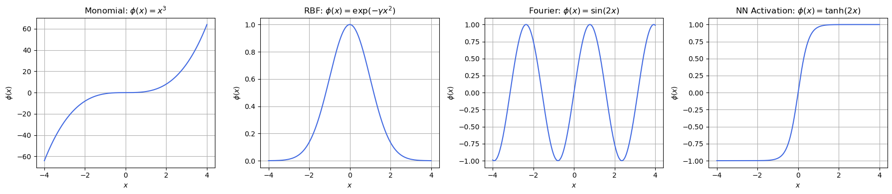
What This Shows:

Feature	Behavior
$x^{3}$	Nonlinear, unbounded, odd symmetry
$\exp (- γ x^{2})$	Peak at center, decays rapidly — localized
$\sin (2 x)$	Periodic — captures repeating structure
$\tanh (2 x)$	S-shaped, saturates for large

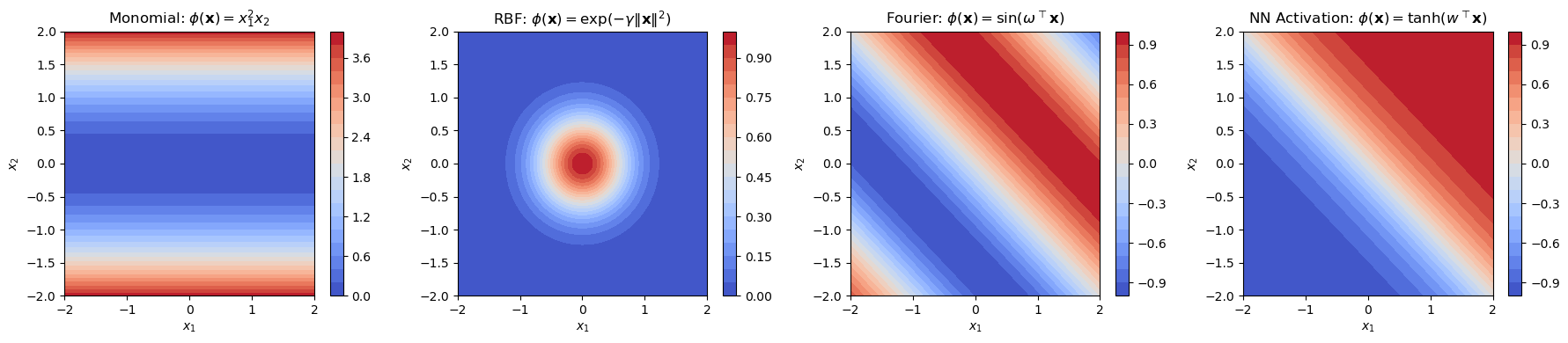
Here is a each type of function plotted over a 2D input space $x = [x_{1}, x_{2}]$ :

../_images/e8c7cf400a25adc30d32936ae987f992c81bb4b3e1abd3e049e015cb353e64d5.png

Basis Functions $ϕ_{j}$	Space $V_{Φ}$ Represents	Used In
Monomials	Polynomial function space $P_{n}^{d}$	Polynomial regression, SVMs
RBFs	Radial function space	RBF kernel SVM, RBF networks
Sinusoids	Fourier basis (periodic functions)	Fourier analysis, signal processing
Neural activations	Neural network hypothesis space	MLPs, deep learning

Example: Multivariate Polynomials in $R^{2}$ #

We start with an example in $R^{2}$ that makes the theoretical concept more tangible.

Let’s consider the space $P_{2}^{2}$ , i.e., all real-valued polynomials in two variables $x_{1}, x_{2}$ of total degree at most 2.

We write $x = [x_{1}, x_{2}] \in R^{2}$ , and we’re interested in all polynomials of the form:

p (x) = a_{00} + a_{10} x_{1} + a_{01} x_{2} + a_{20} x_{1}^{2} + a_{11} x_{1} x_{2} + a_{02} x_{2}^{2}

Where each $a_{i j} \in R$ , and the total degree of each monomial (i.e., $i + j$ ) is at most 2.

Basis for $P_{2}^{2}$ #

A natural basis for this space is the set of monomials:

{1, x_{1}, x_{2}, x_{1}^{2}, x_{1} x_{2}, x_{2}^{2}}

So, $\dim P_{2}^{2} = 6$ , and every element of $P_{2}^{2}$ is a linear combination of these basis monomials.

Example Polynomial#

Let’s define:

p (x) = 3 + 2 x_{1} - x_{2} + 5 x_{1} x_{2} - x_{2}^{2}

This polynomial is clearly in $P_{2}^{2}$ because:

All monomials are of total degree ≤ 2.
The coefficients $[3, 2, - 1, 0, 5, - 1]$ match the basis ordering.

Vector Space Properties (concretely)#

Addition: If we add two such polynomials, we just add their coefficients.
Scalar multiplication: Scaling multiplies all coefficients.
Zero element: The polynomial $0 = 0 + 0 x_{1} + 0 x_{2} + 0 x_{1}^{2} + 0 x_{1} x_{2} + 0 x_{2}^{2}$
Inverse: Negate each coefficient.

Polynomial Features in Machine Learning#

Using polynomial vector spaces, we can enhance simple machine learning algorithms by explicitly representing complex, nonlinear relationships. We will use the Nearest Centroid Classifier, a linear classifier that classifies samples based on their distance to the centroid of each class. This classifier is simple yet effective, especially when combined with basis functions.

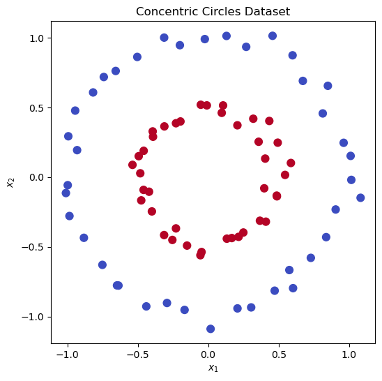
Let’s look at a challenging synthetic sata set, the “concentric circles” dataset that contains two classes arranged as points along concentric circles of different radius that are not linearly separable in the original space.

../_images/25f7ead5a63f5448c9bf3199525262956f81f4bd0ea32c6e93a7516e8f5832dd.png

The space $P_{2}^{2}$ gives you a natural feature map to transform the data into a higher-dimensional space where the classes may become linearly separable. The transformation is defined as:

ϕ : R^{2} \to R^{6}, x \mapsto [1, x_{1}, x_{2}, x_{1}^{2}, x_{1} x_{2}, x_{2}^{2}]

Let’s visualize the transformation of the concentric circles dataset using polynomial features up to degree 2.

../_images/28f459758f346071be4c9532a54ef4a814e195f39c6892a37493346a539cf182.png

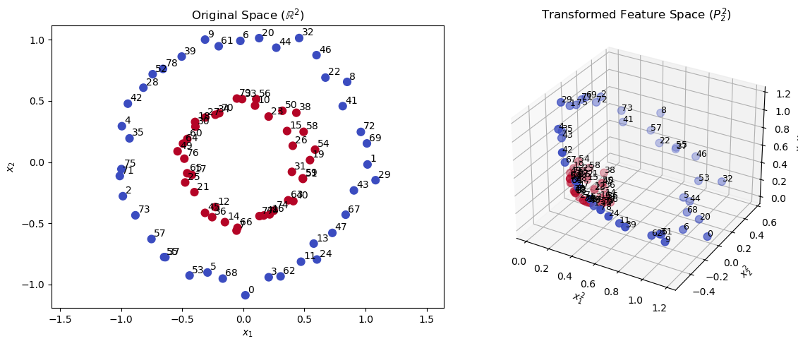
We see that in the additional dimensions in the transformed space $P_{2}^{2}$ (right), the data points are more spread out and the clusters become linearly separable. So, let’s apply the Nearest Centroid Classifier to the original and the transformed data.

../_images/3dbc7789f8c74cc64e4df65c4616d4e480c09e84ad9c120fb9d33c14aacd3cfc.png

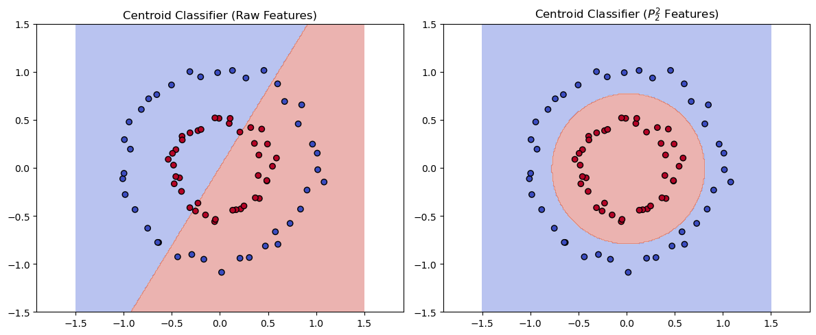
The left plot shows the decision boundary of the Nearest Centroid Classifier using the original features, while the right plot shows the decision boundary after applying polynomial feature expansion. The polynomial transformation allows the classifier to separate the classes effectively. Note that the Nearest Centroid classifier is a linear classifier. While the decision boundary forms a circle in the original space $R^{2}$ , it is a flat hyperplane in the transformed space. This is a key point when using non-linear basis functions in the context of linear machine learning methods: Learned functions are linear in the transformed space, but can be nonlinear in the original space.

Further Examples (Moons + XOR)#

Let’s also compare the polynomial $P_{2}^{2}$ transformation to the Radial Basis Function (RBF) transformation and add two more challenging datasets: the Two Moons and XOR datasets.

The Two Moons dataset consists of two interleaving half circles, while the XOR dataset consists of four points arranged in a square pattern. Both datasets are not linearly separable in their original feature space.

Show code cell source Hide code cell source

import numpy as np
import matplotlib.pyplot as plt
from sklearn.datasets import make_circles, make_moons
from sklearn.neighbors import NearestCentroid
from sklearn.preprocessing import StandardScaler

# --- RBF centers: grid over input space
grid_centers = np.array([[x, y] for x in np.linspace(-2, 2, 5) for y in np.linspace(-2, 2, 5)])

# --- Dataset 1: Concentric Circles ---
X0, y0 = make_circles(n_samples=80, factor=0.5, noise=0.1, random_state=42)
X0 = StandardScaler().fit_transform(X0)

# --- Dataset 2: Two Moons ---
X1, y1 = make_moons(n_samples=80, noise=0.05, random_state=1)
X1 = StandardScaler().fit_transform(X1)

# --- Dataset 3: XOR pattern ---
X2_base = np.array([[0, 0], [1, 1], [0, 1], [1, 0]]) * 2 - 1
y2_base = np.array([0, 0, 1, 1])
X2 = np.tile(X2_base, (20, 1)) + np.random.normal(scale=0.2, size=(80, 2))
y2 = np.tile(y2_base, 20)
X2 = StandardScaler().fit_transform(X2)

datasets = [
    ("Circles", X0, y0),
    ("Two Moons", X1, y1),
    ("XOR", X2, y2)
]

# --- Plotting ---
fig, axes = plt.subplots(3, 3, figsize=(15, 15))

for i, (name, X, y) in enumerate(datasets):
    # Raw model
    model_raw = NearestCentroid()
    model_raw.fit(X, y)

    # Polynomial model
    X_poly = monomial_features(X, max_degree=2)
    model_poly = NearestCentroid()
    model_poly.fit(X_poly, y)

    # RBF model
    X_rbf = rbf_features(X, grid_centers, gamma=2.0)
    model_rbf = NearestCentroid()
    model_rbf.fit(X_rbf, y)

    # Grid for visualization
    xx, yy = np.meshgrid(np.linspace(-2, 2, 300),
                         np.linspace(-2, 2, 300))
    grid = np.c_[xx.ravel(), yy.ravel()]
    grid_poly = monomial_features(grid, max_degree=2)
    grid_rbf = rbf_features(grid, grid_centers, gamma=2.0)

    # Predictions
    Z_raw = model_raw.predict(grid).reshape(xx.shape)
    Z_poly = model_poly.predict(grid_poly).reshape(xx.shape)
    Z_rbf = model_rbf.predict(grid_rbf).reshape(xx.shape)

    # --- Plot Raw ---
    axes[i, 0].contourf(xx, yy, Z_raw, alpha=0.4, cmap='coolwarm')
    axes[i, 0].scatter(X[:, 0], X[:, 1], c=y, edgecolor='k', cmap='coolwarm')
    axes[i, 0].set_title(f"{name} - Raw Features")
    axes[i, 0].axis('equal')

    # --- Plot Polynomial ---
    axes[i, 1].contourf(xx, yy, Z_poly, alpha=0.4, cmap='coolwarm')
    axes[i, 1].scatter(X[:, 0], X[:, 1], c=y, edgecolor='k', cmap='coolwarm')
    axes[i, 1].set_title(f"{name} - $P_2^2$ Features")
    axes[i, 1].axis('equal')

    # --- Plot RBF ---
    axes[i, 2].contourf(xx, yy, Z_rbf, alpha=0.4, cmap='coolwarm')
    axes[i, 2].scatter(X[:, 0], X[:, 1], c=y, edgecolor='k', cmap='coolwarm')
    axes[i, 2].set_title(f"{name} - RBF Features")
    axes[i, 2].axis('equal')

plt.tight_layout()
plt.show()

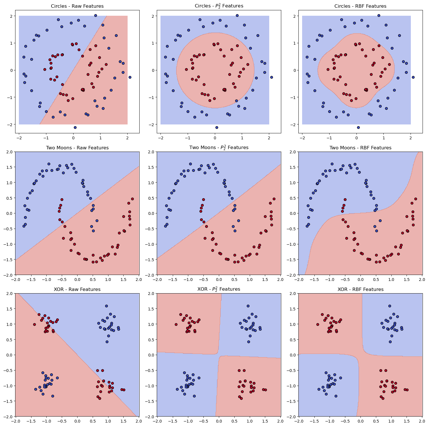
../_images/57f06ac7cb49e50f9f3d32554fcd96a0f1697f6089c3f7c1a7b78dfdc031a754.png

We see that both feature transformations perform well on the concentric circles dataset and the XOR dataset, but the polynomial features are not as effective on the two moons dataset as the RBF features, which can capture the local structure of the data.