Vectors, Functions and the Spaces they live in#
In this chapter we present important classes of spaces in which our data will live and our operations will take place: vector spaces, metric spaces, normed spaces, and inner product spaces. Generally speaking, these are defined in such a way as to capture one or more important properties of Euclidean space but in a more general way. Classical Euclidean spaces that in machine learning are most commonly used to model the inputs and outputs of a machine learning algorithm are finite-dimensional. Functions on the other hand are not finite-dimensional, and in fact, most of the spaces we will be working with are often infinite-dimensional. Functions are the most common objects in these infinite-dimensional spaces, and we will see that they can be treated as vectors.
Vectors and functions, though seemingly different, share many common properties by virtue of inhabiting vector spaces. In a finite-dimensional vector space like \(\mathbb{R}^n\), vectors are ordered tuples of numbers that can be easily visualized as points or arrows in Euclidean space. They obey the familiar rules of addition and scalar multiplication, which makes them very intuitive to work with. Functions, on the other hand, are objects that map inputs to outputs and generally reside in infinite-dimensional spaces. Despite this, many function spaces also exhibit vector space structure; for instance, if \(f\) and \(g\) are functions, then so is \(\alpha f + \beta g\) for any scalars \(\alpha, \beta\). In machine learning, this duality is essential: finite-dimensional vectors often represent data points or feature vectors, while functions are used to model predictions, transformations, or the behavior of learning algorithms. Although the infinite-dimensional nature of function spaces might seem more complex, by choosing an appropriate basis (such as Fourier or wavelet bases) one can often work with finite-dimensional approximations of these function spaces. This common structure allows us to use similar mathematical tools—like inner products, norms, and projections—to analyze both data and models, thereby bridging the gap between concrete numerical computations and abstract function estimation.
Show code cell source
import numpy as np
import matplotlib.pyplot as plt

# Create a figure with two subplots: one for a finite-dimensional vector space and one for function space.
fig, axs = plt.subplots(1, 2, figsize=(14, 6))

### Left Subplot: Finite-Dimensional Vector Space Example
# Example: Visualizing vectors in R².
origin = np.array([0, 0])
# Define a few example vectors in R^2.
vectors = np.array([[2, 1],
                    [1, 2],
                    [-1, 1],
                    [-2, -1]])

# Plot each vector as an arrow originating from the origin.
for vec in vectors:
    axs[0].quiver(origin[0], origin[1], vec[0], vec[1], angles='xy', scale_units='xy', scale=1, color='blue')

# Setup plot aesthetics.
axs[0].set_xlim(-3, 3)
axs[0].set_ylim(-3, 3)
axs[0].set_title("Finite-Dimensional Vector Space (R²)")
axs[0].set_xlabel("X₁")
axs[0].set_ylabel("X₂")
axs[0].grid(True)
axs[0].axhline(0, color='black', lw=0.5)
axs[0].axvline(0, color='black', lw=0.5)

### Right Subplot: Function Space Example
# In a function space, functions can be represented as "vectors" via their coefficients in a chosen basis.
# For illustration, approximate a function in L²[0, 2π] using a simple basis of sinusoids.
x = np.linspace(0, 2*np.pi, 400)
# Define a target function as a linear combination of basis functions.
f_target = 1.5 * np.sin(x) + 0.5 * np.cos(2*x)
# Basis functions (for illustrative purposes).
phi1 = np.sin(x)
phi2 = np.cos(x)
phi3 = np.cos(2*x)
# The approximated function using specific coefficients corresponds to a point (vector) of coefficients in the finite-dimensional approximation.
f_approx = 1.5 * phi1 + 0.0 * phi2 + 0.5 * phi3

# Plot the target function and the basis functions.
axs[1].plot(x, f_target, label="Target Function", color="blue", linewidth=2)
axs[1].plot(x, phi1, label="Basis: sin(x)", linestyle='--', color="gray")
axs[1].plot(x, phi2, label="Basis: cos(x)", linestyle='--', color="orange")
axs[1].plot(x, phi3, label="Basis: cos(2x)", linestyle='--', color="green")
# Plot the approximated function as the result of the linear combination.
axs[1].plot(x, f_approx, label="Approximated Function", color="red", linewidth=2)

# Setup plot aesthetics.
axs[1].set_title("Function Space Representation")
axs[1].set_xlabel("x")
axs[1].set_ylabel("f(x)")
axs[1].grid(True)
axs[1].legend(loc="upper right", fontsize=8)

plt.suptitle("Illustration: Vectors vs. Functions in Their Respective Vector Spaces", fontsize=16)
plt.tight_layout(rect=[0, 0.03, 1, 0.95])
plt.show()
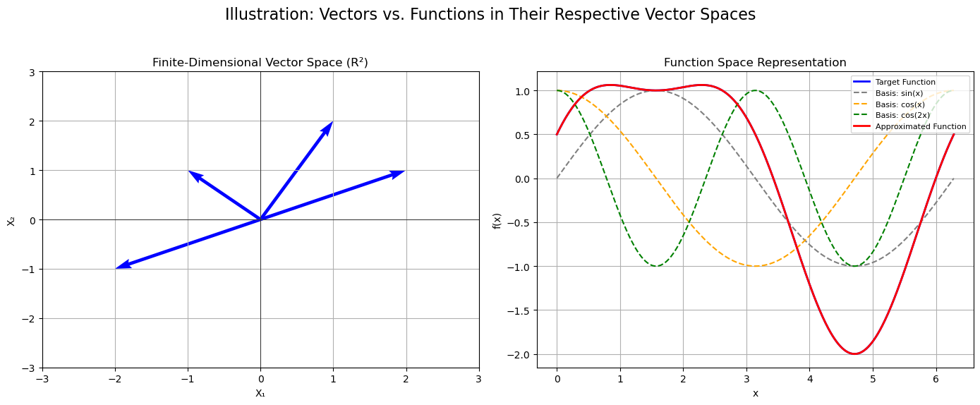
Left Plot (Finite-Dimensional Vector Space):
The left subplot displays several arrows representing vectors in \(\mathbb{R}^2\). Each vector is an element of a finite-dimensional space (with just two components), and the operations (addition, scalar multiplication) on these vectors are straightforward and visualizable.Right Plot (Function Space):
The right subplot illustrates a function \(f(x)\) as a curve over the interval \([0, 2\pi]\). Although function spaces are inherently infinite-dimensional, we approximate them by representing functions in a finite basis (here, using sinusoids). The target function is expressed as a linear combination of basis functions, and the approximated function (in red) is determined by specific coefficients. This demonstrates how functions can be treated as vectors in a finite-dimensional subspace of an infinite-dimensional function space.