Regression#
Regression is a supervised learning task focused on predicting continuous numeric values rather than discrete categories. Common regression tasks include predicting the price of a house, forecasting weather conditions, estimating the age of a person from an image, or determining the severity of a disease based on medical test results.
In regression, we are given pairs of \((\mathbf{x}, y)\), the so-called training data and we would like to train a function \(f(\mathbf{x})\) that predicts a continuous value of \(y\in\mathbb{R}\).
Inputs: A collection of feature vectors, typically represented as vectors in a vector space, for example Euclidean space:
Targets: Each feature vector is assigned a label from a finite set of categories, often represented as:
The aim is to learn a mathematical function \(f(\mathbf{x})\) that maps input features to continuous predictions of the target variable \(y\):
The difference between the targets and the predictions is called the error or residual \(\epsilon\). The goal of regression is to minimize this error across all training samples.
Regression of temperature data from Potsdam#
To illustrate regression, we will look at with weather data collected from the station in Potsdam, distributed by the DAILY GLOBAL HISTORICAL CLIMATOLOGY NETWORK (GHCN-DAILY) [1].
The dataset consists of daily weather data recorded in Potsdam Babelsberg from January 1st, 1893 up to January 30th, 2024 [2,3].
Linear Regression: A foundational example#
The simplest and most fundamental regression model is linear regression, which assumes that the relationship between input features and the output target is linear:
Here, \(\mathbf{w}\) is a vector of weights and \(b\) is a bias (intercept) term. To find the best-fit model, linear regression minimizes the squared differences between observed and predicted values (the mean squared error):
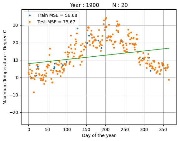
Let’s use linear regression to predict the maximum temperature \(t_\mathrm{max}\) for a given day of the year 2000.
Where:
\(t_{max}\) is the maximum temperature for a given day
\(w\) is the slope (average temperature change per day)
\(b\) is the intercept (base temperature)
\(x\) is the day in the year (0-365)
Show code cell source
import numpy as np
import pandas as pd
import matplotlib.pyplot as plt
YEAR = 1900
def load_weather_data(year = None):
    """
    load data from a weather station in Potsdam
    """

    names = ['station', 'date' , 'type', 'measurement', 'e1','e2', 'E', 'e3']
    data = pd.read_csv('../../datasets/weatherstations/GM000003342.csv', names = names, low_memory=False) # 47876 rows, 8 columns
    # convert the date column to datetime format
    data['date'] = pd.to_datetime(data['date'], format="%Y%m%d") # 47876 unique days
    types = data['type'].unique()

    tmax = data[data['type']=='TMAX'][['date','measurement']] # Maximum temperature (tenths of degrees C), 47876
    tmin = data[data['type']=='TMIN'][['date','measurement']] # Minimum temperature (tenths of degrees C), 47876
    prcp = data[data['type']=='PRCP'][['date','measurement']] # Precipitation (tenths of mm), 47876
    snwd = data[data['type']=='SNWD'][['date','measurement']] # Snow depth (mm), different shape
    tavg = data[data['type']=='TAVG'][['date','measurement']] # average temperature, different shape 1386
    arr = np.array([tmax.measurement.values,tmin.measurement.values, prcp.measurement.values]).T

    df = pd.DataFrame(arr/10.0, index=tmin.date, columns=['TMAX', 'TMIN', 'PRCP']) # compile data in a dataframe and convert temperatures to degrees C, precipitation to mm

    if year is not None:
        df = df[pd.to_datetime(f'{year}-1-1'):pd.to_datetime(f'{year}-12-31')]

    df['days'] = (df.index - df.index.min()).days
    return df

class UnivariateLinearRegression:
    def __init__(self):
        self.x = None
        self.y = None
        self.w = None
        self.b = None

    def train(self, x, y):
        self.x = x
        self.y = y
        self.w = np.sum((x - np.mean(x)) * (y - np.mean(y))) / np.sum((x - np.mean(x))**2)
        self.b = np.mean(y) - self.w * np.mean(x)

    def pred(self, x):
        y = self.w * x + self.b
        return y

    def mse(self, x=None, y=None):
        if x is None:
            x = self.x
        if y is None:
            y = self.y
        y_pred = self.pred(x)
        mse = np.mean((y - y_pred)**2)
        return mse

    def score(self, x=None, y=None):
        return -self.mse(x, y)

# Load weather data for the year 2000
df = load_weather_data(year = YEAR)

np.random.seed(2)
idx = np.random.permutation(df.shape[0])

idx_train = idx[0:100]
idx_test = idx[100:]

data_train = df.iloc[idx_train]
data_test = df.iloc[idx_test]

N_train = 20

x_train = data_train.days.values[:N_train] * 1.0
y_train = data_train.TMAX.values[:N_train]

reg = UnivariateLinearRegression()
reg.train(x_train, y_train)

x_days = np.arange(366)
y_days_pred = reg.pred(x_days)

x_test = data_test.days.values * 1.0
y_test = data_test.TMAX.values
y_test_pred = reg.pred(x_test)
print("training MSE : %.4f" % reg.mse())
print("test MSE     : %.4f" % reg.mse(x_test, y_test))

fig = plt.figure()
ax = plt.plot(x_train,y_train,'.')
ax = plt.plot(x_test,y_test,'.')
ax = plt.legend(["Train MSE = %.2f" % reg.mse(),"Test MSE = %.2f" % reg.mse(x_test, y_test)])
ax = plt.plot(x_days,y_days_pred)
ax = plt.ylim([-27,39])
ax = plt.xlabel("Day of the year")
ax = plt.ylabel("Maximum Temperature - Degree C")
ax = plt.title("Year : %i        N : %i" % (YEAR, N_train))
ax = plt.grid(True)
training MSE : 56.6761
test MSE     : 75.6696
Beyond Linear Regression#
While linear regression is simple and interpretable, it may struggle with data exhibiting complex, nonlinear relationships such as the non-linear dependency between the day of the year and the temperature. Extensions like polynomial regression or kernel regression introduce nonlinear features or transformations to capture more intricate patterns, while regularization techniques such as ridge regression or the use of Bayesian linear regression help control model complexity and prevent overfitting.
Show code cell source
class RidgeRegression:
    """
    Ridge Regression model.

    Attributes:
        ridge (float): Regularization parameter.
        N (int): Number of samples.
        w (numpy.ndarray): Coefficients of the fitted model.
        fit_mean (bool): Whether to fit the mean of the data.
    """
    def __init__(self, ridge=0.0, fit_mean=False):
        """
        Initializes the KernelRidgeRegression model with specified parameters.

        Args:
            ridge (float, optional): Regularization parameter. Defaults to 0.0.
            fit_mean (bool, optional): Whether to fit the mean of the data. Defaults to False.
        """
        self.ridge = ridge
        self.N = None
        self.w = None
        self.fit_mean = fit_mean

    def fit(self, X, y):
        """
        Fits the model to the training data.

        Args:
            X (numpy.ndarray): Training feature design matrix.
            y (numpy.ndarray): Target variable.

        Notes:
            The method computes the coefficients of the model using the provided kernel matrix and target variable.
        """
        if self.fit_mean:
            self.mean_y = y.mean(0)
            self.mean_X = X.mean(0)
            X = X - self.mean_X[np.newaxis,:]
            y = y - self.mean_y
        else:
            self.mean_y = 0.0
        self.N = X.shape[0]
        XX = X.T @ X + np.eye(X.shape[1]) * self.ridge
        Xy = X.T @ y
        self.w = np.linalg.lstsq(XX, Xy, rcond=None)[0]

    def pred(self, X_star):
        """
        Predicts target variable for new data.

        Args:
            X_star (numpy.ndarray): Feature design matrix for new data.

        Returns:
            numpy.ndarray: Predicted target variable.
        """
        if self.fit_mean:
            X_star = X_star - self.mean_X[np.newaxis,:]
        return X_star @ self.w + self.mean_y

    def mse(self, X, y):
        """
        Computes mean squared error.

        Args:
            X (numpy.ndarray): Feature design matrix.
            y (numpy.ndarray): Target variable.

        Returns:
            float: Mean squared error.
        """
        y_pred = self.pred(X)
        residual = y - y_pred
        return np.mean(residual * residual)

    def score(self, X, y):
        """
        Computes the score of the model.

        Args:
            X (numpy.ndarray): Feature design matrix.
            y (numpy.ndarray): Target variable.

        Returns:
            float: Score of the model.
        """
        return self.mse(X=X, y=y)

fit_mean = True     # fit a separate mean for y in the linear regression?
ridge = 0     # strength of the L2 penalty in ridge regression

x_train = data_train.days.values[:N_train][:,np.newaxis] * 1.0
X_train = np.concatenate((x_train,x_train*x_train),1)
y_train = data_train.TMAX.values[:N_train]

reg = RidgeRegression(fit_mean=fit_mean, ridge=ridge)
reg.fit(X_train, y_train)

x_days = np.arange(366)[:,np.newaxis]
X_days = np.concatenate((x_days,x_days*x_days),1)
y_days_pred = reg.pred(X_days)

x_test = data_test.days.values[:,np.newaxis] * 1.0
X_test = np.concatenate((x_test,x_test*x_test),1)
y_test = data_test.TMAX.values
y_test_pred = reg.pred(X_test)
print("training MSE : %.4f" % reg.mse(X_train, y_train))
print("test MSE     : %.4f" % reg.mse(X_test, y_test))


fig = plt.figure()
ax = plt.plot(x_train,y_train,'.')
ax = plt.plot(x_test,y_test,'.')
ax = plt.legend(["train MSE = %.2f" % reg.mse(X_train, y_train),"test MSE = %.2f" % reg.mse(X_test, y_test)])
ax = plt.plot(x_days,y_days_pred)
ax = plt.ylim([-27,39])
ax = plt.xlabel("day of the year")
ax = plt.ylabel("Maximum Temperature - degree C")
ax = plt.title("Year : %i        N : %i" % (YEAR, N_train))
training MSE : 17.3267
test MSE     : 28.7596
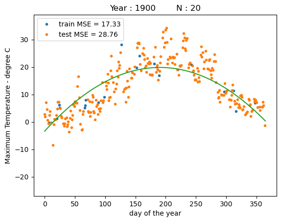
We can see that a polynomial regression model with a second order polynomial (quadratic) can fit the data much better than a linear regression model.
Examples of regression algorithms covered in this book:#
Linear Regression: Fundamental regression method illustrating vector spaces, inner products, and optimization basics.
Polynomial Regression: Uses polynomial features to model nonlinear relationships, demonstrating vector spaces formed by polynomial bases.
Ridge Regression: Incorporates L2 regularization (vector norms) to prevent overfitting.
Bayesian Linear Regression: Combines probabilistic modeling and linear algebra, providing uncertainty estimates for predictions.
Gaussian Processes: Nonparametric regression method using covariance functions to model complex relationships, showcasing advanced linear algebra concepts.
In the chapters ahead, regression tasks will serve as a powerful motivation to explore concepts in linear algebra (vector spaces, norms, matrix decompositions), calculus and optimization (gradient descent and second-order methods), and probability (Gaussian distributions, covariance estimation, and Bayesian inference). Understanding these mathematical foundations will equip you to build effective, robust, and interpretable regression models.
References#
[1] Menne, M.J., I. Durre, R.S. Vose, B.E. Gleason, and T.G. Houston, 2012: An overview of the Global Historical Climatology Network-Daily Database. Journal of Atmospheric and Oceanic Technology, 29, 897-910, doi:10.1175/JTECH-D-11-00103.1.
[2] Menne, M.J., I. Durre, B. Korzeniewski, S. McNeal, K. Thomas, X. Yin, S. Anthony, R. Ray, R.S. Vose, B.E.Gleason, and T.G. Houston, 2012: Global Historical Climatology Network - Daily (GHCN-Daily), Version 3. [indicate subset used following decimal, e.g. Version 3.12]. NOAA National Climatic Data Center. http://doi.org/10.7289/V5D21VHZ [2024/01/31].
[3] Klein Tank, A.M.G. and Coauthors, 2002. Daily dataset of 20th-century surface air temperature and precipitation series for the European Climate Assessment. Int. J. of Climatol., 22, 1441-1453. Data and metadata available at http://eca.knmi.nl