Transposition#
If \(\mathbf{A} \in \mathbb{R}^{m \times n}\), its transpose \(\mathbf{A}^{\!\top\!} \in \mathbb{R}^{n \times m}\) is given by \((\mathbf{A}^{\!\top\!})_{ij} = A_{ji}\) for each \((i, j)\). In other words, the columns of \(\mathbf{A}\) become the rows of \(\mathbf{A}^{\!\top\!}\), and the rows of \(\mathbf{A}\) become the columns of \(\mathbf{A}^{\!\top\!}\).
The transpose has several nice algebraic properties that can be easily verified from the definition:
(i) \((\mathbf{A}^{\!\top\!})^{\!\top\!} = \mathbf{A}\)
(ii) \((\mathbf{A}+\mathbf{B})^{\!\top\!} = \mathbf{A}^{\!\top\!} + \mathbf{B}^{\!\top\!}\)
(iii) \((\alpha \mathbf{A})^{\!\top\!} = \alpha \mathbf{A}^{\!\top\!}\)
(iv) \((\mathbf{A}\mathbf{B})^{\!\top\!} = \mathbf{B}^{\!\top\!} \mathbf{A}^{\!\top\!}\)
ML Example: Efficient Kernel Computation Using Transposition Rules#
Kernel methods in machine learning often require efficiently computing similarity between data points. Let’s see clearly how transposition helps simplify the calculation of kernels, specifically the Polynomial kernel and the RBF (Gaussian) kernel.
Consider data stored in a matrix form:
\(\mathbf{X} \in \mathbb{R}^{m \times n}\), representing \(m\) data points (rows), each with \(n\) features (columns).
Example 1: Efficient Polynomial Kernel Computation#
Recall the polynomial kernel of degree \(d\):
We can compute the entire polynomial kernel matrix \(\mathbf{K}\) between all pairs of data points efficiently using matrix transposition:
Define \(\mathbf{K}_{\text{poly}}\) as:
Here:
\(\mathbf{X}\mathbf{X}^{\!\top\!}\) efficiently computes all pairwise dot products between data points.
\((\,\cdot\,)^{\circ d}\) means element-wise exponentiation to the power of \(d\).
Transposition explicitly used:#
\((\mathbf{X}\mathbf{X}^{\!\top\!})_{ij}\) represents the dot product between data points \(\mathbf{x}_i\) and \(\mathbf{x}_j\).
Thus, transposition helps in neatly representing pairwise inner products.
Example 2: Efficient Gaussian (RBF) Kernel Computation#
Recall the Gaussian (RBF) kernel:
At first glance, computing all pairwise squared distances can look computationally expensive. Using transposition rules, we simplify this expression:
Note first that:
Thus, the kernel matrix \(\mathbf{K}_{\text{RBF}}\) is efficiently computed for all pairs simultaneously using matrix transposition:
Compute vector of squared norms for all data points:
Compute the full squared-distance matrix using broadcasting:
Here:
\(\mathbf{1}\) is an \(m\times 1\) vector of ones.
Each element \(D_{ij}\) corresponds to the squared Euclidean distance between \(\mathbf{x}_i\) and \(\mathbf{x}_j\).
Finally, the RBF kernel matrix is:
Transposition explicitly used:#
The simplification \((\mathbf{x}-\mathbf{y})^{\!\top\!}(\mathbf{x}-\mathbf{y})\) explicitly leverages transposition rules.
The compact and computationally efficient matrix notation relies on careful application of transposition to simplify algebraic expressions.
Why this matters:#
Transposition rules provide a clean, computationally efficient way of expressing kernel computations.
Even without introducing complex concepts like covariance or gradients, students clearly see the utility of transposition in practical ML settings (e.g., kernel methods).
Demonstrates the algebraic elegance and computational importance of linear algebra fundamentals early in their ML education.
Quick reference to transposition rules used:#
Property |
Usage |
|---|---|
\((\mathbf{A}\mathbf{B})^{\!\top\!} = \mathbf{B}^{\!\top\!}\mathbf{A}^{\!\top\!}\) |
Simplifying inner product expressions |
\((\mathbf{A}^{\!\top\!})^{\!\top\!} = \mathbf{A}\) |
Simplifying algebraic expressions clearly |
Below is a complete Python script that demonstrates how to compute kernel matrices efficiently using transposition rules. In this example, we work with a synthetic data matrix \(\mathbf{X} \in \mathbb{R}^{m \times n}\) and show:
How to compute the polynomial kernel matrix by using \(\mathbf{X}\mathbf{X}^{\top}\) (which yields all pairwise dot products) and then applying an element‐wise power.
How to compute the Gaussian (RBF) kernel matrix by using transposition to first compute the squared Euclidean distances between all pairs.
The script then visualizes both kernel matrices using heatmaps.
Show code cell source
import numpy as np
import matplotlib.pyplot as plt
# --------------------------
# Generate synthetic data
# --------------------------
# Let m be the number of data points and n be the number of features.
m, n = 10, 5
np.random.seed(42)
X = np.random.randn(m, n) # Data matrix: each row is a data point in R^n
# --------------------------
# Example 1: Polynomial Kernel
# --------------------------
# The polynomial kernel of degree d with constant c is defined as:
# k_poly(x,y) = (x^T y + c)^d
# We compute the entire kernel matrix for X using:
# K_poly = (X X^T + c) ^{circ d}
c = 1.0 # Constant term
d = 3 # Degree of the polynomial
# Compute X X^T using matrix multiplication (using the transposition property)
XXT = X @ X.T # XXT is an m x m matrix with (i,j)-th entry = <x_i, x_j>
# Add constant c to each element and perform element-wise exponentiation to the power d
K_poly = (XXT + c) ** d
# --------------------------
# Example 2: Gaussian (RBF) Kernel
# --------------------------
# The Gaussian (RBF) kernel is defined as:
# k_RBF(x,y) = exp(-γ || x - y||^2 )
# and we can use transposition to compute the squared Euclidean distances efficiently.
gamma = 0.5 # Parameter for the RBF kernel
# Step 1: Compute the squared norms for all data points using the diagonal of XXT.
squared_norms = np.diag(XXT) # shape: (m,)
# Step 2: Compute the squared Euclidean distance matrix D using broadcasting.
# Each element D[i,j] is:
# ||x_i - x_j||^2 = <x_i, x_i> - 2<x_i, x_j> + <x_j, x_j>
D = squared_norms.reshape(-1, 1) - 2 * XXT + squared_norms.reshape(1, -1)
# Step 3: Compute the RBF kernel matrix.
K_RBF = np.exp(-gamma * D)
# --------------------------
# Visualization of the Kernel Matrices
# --------------------------
fig, axs = plt.subplots(1, 2, figsize=(14, 6))
# Polynomial Kernel Heatmap
im0 = axs[0].imshow(K_poly, cmap='viridis', aspect='equal')
axs[0].set_title(f"Polynomial Kernel (degree {d}, c={c})")
axs[0].set_xlabel("Data Point Index")
axs[0].set_ylabel("Data Point Index")
plt.colorbar(im0, ax=axs[0], fraction=0.046, pad=0.04)
# RBF Kernel Heatmap
im1 = axs[1].imshow(K_RBF, cmap='viridis', aspect='equal')
axs[1].set_title(f"Gaussian (RBF) Kernel (gamma={gamma})")
axs[1].set_xlabel("Data Point Index")
axs[1].set_ylabel("Data Point Index")
plt.colorbar(im1, ax=axs[1], fraction=0.046, pad=0.04)
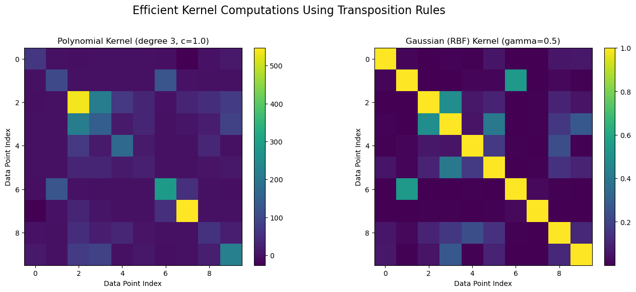
plt.suptitle("Efficient Kernel Computations Using Transposition Rules", fontsize=16)
plt.tight_layout(rect=[0, 0.03, 1, 0.95])
plt.show()
Explanation#
Polynomial Kernel Computation:
We compute the matrix \( \mathbf{X}\mathbf{X}^{\top} \) to obtain all pairwise dot products.
Adding a constant \(c\) and then taking an element-wise power \(d\) yields the polynomial kernel matrix: $\( \mathbf{K}_{\text{poly}} = (\mathbf{X}\mathbf{X}^{\top} + c)^{\circ d}. \)$
Transposition is essential in \(\mathbf{X}\mathbf{X}^{\top}\) since it converts the \(n\)-dimensional row vectors into column vectors to perform the dot products.
Gaussian (RBF) Kernel Computation:
The vector of squared norms is extracted from the diagonal of \(\mathbf{X}\mathbf{X}^{\top}\).
The squared distance matrix is computed using the formula: $\( D_{ij} = \|\mathbf{x}_i - \mathbf{x}_j\|^2 = \mathbf{x}_i^\top \mathbf{x}_i - 2 \mathbf{x}_i^\top \mathbf{x}_j + \mathbf{x}_j^\top \mathbf{x}_j. \)$
Finally, the RBF kernel matrix is obtained by applying the exponential function with parameter \(\gamma\).
Visualization:
Two subplots display the kernel matrices as heatmaps, clearly demonstrating the efficiency of using transposition rules for kernel computation.
The colorbars help to interpret the relative similarities between data points as computed by the kernels.
This script ties together linear algebra (via transposition) and practical kernel methods in machine learning, highlighting how fundamental operations can lead to efficient and elegant implementations.