Polynomials#
In the previous sections, we have explored the properties of finite-dimensional vector spaces, focusing on the familiar Euclidean spaces \(\mathbb{R}^n\). These spaces are characterized by their finite number of dimensions and the operations of vector addition and scalar multiplication. However, as we delve deeper into the world of machine learning and functional analysis, we encounter a new realm: infinite-dimensional function spaces. These spaces are more complex and abstract than their finite-dimensional counterparts, yet they play a crucial role in understanding various machine learning algorithms and models.
To bridge our understanding from finite-dimensional Euclidean spaces to infinite-dimensional function spaces, we begin with one of the simplest families of functions that still form a vector space: polynomials. Polynomials in one variable of bounded degree provide a gentle first step into function spaces because, despite being functions, they can be fully described using a finite number of real-valued coefficients. Just like vectors in \(\mathbb{R}^n\), polynomials of degree at most \(n\) form a vector space—every linear combination of polynomials of degree \(\leq n\) is again a polynomial of degree \(\leq n\). This makes them ideal for illustrating how familiar vector operations extend to function spaces. In machine learning, polynomials appear naturally in regression problems, where they are used to approximate non-linear relationships in data while retaining the interpretability and structure of linear models. As we will see, learning polynomial models is equivalent to performing linear regression in a transformed, higher-dimensional feature space—an idea that lies at the heart of many modern learning algorithms.
Polynomial Basis Functions#
Show code cell source
import numpy as np
import matplotlib.pyplot as plt

# Create a grid of x values
x = np.linspace(-1, 1, 300)

# Define the basis polynomials
phi0 = np.ones_like(x)        # x^0
phi1 = x                      # x^1
phi2 = x**2                   # x^2
phi3 = x**3                   # x^3

# Set up the plot
plt.figure(figsize=(10, 6))

# Plot each polynomial basis function
plt.plot(x, phi0, label=r"$\phi_0(x) = x^0$", linestyle="--")
plt.plot(x, phi1, label=r"$\phi_1(x) = x^1$", linestyle="-.")
plt.plot(x, phi2, label=r"$\phi_2(x) = x^2$", linestyle=":")
plt.plot(x, phi3, label=r"$\phi_3(x) = x^3$", linestyle="-")

# Decorate the plot
plt.title("Polynomial Basis Functions (Monomials)", fontsize=14)
plt.xlabel("x", fontsize=12)
plt.ylabel("Function value", fontsize=12)
plt.grid(True, linestyle=':')
plt.axhline(0, color="black", linewidth=0.5)
plt.axvline(0, color="black", linewidth=0.5)
plt.legend()
plt.tight_layout()
plt.show()
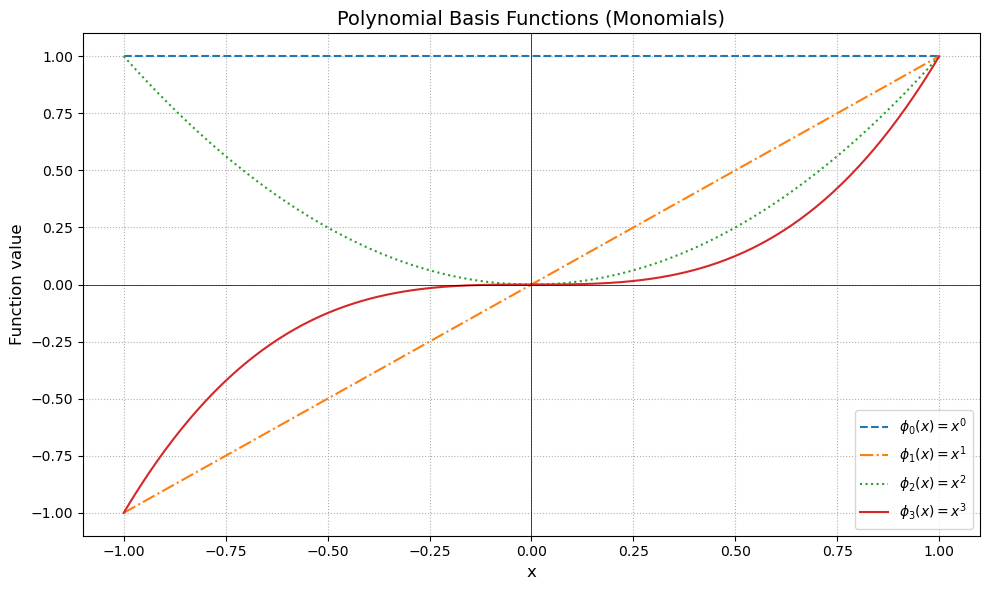
Each curve represents a basis function (monomial) for the space of polynomials \( P_3 \).
Just like unit vectors span directions in \(\mathbb{R}^n\), these functions span a 4-dimensional vector space of degree-3 polynomials.
Any polynomial \( p(x) = a_0 + a_1 x + a_2 x^2 + a_3 x^3 \) is a linear combination of these basis functions.
Polynomial Vector Space#
The vector space of polynomials provides useful tools for machine learning. We will show that the set of all polynomials of degree at most \(n\) forms a vector space. We will also discuss polynomial regression, a powerful technique for modeling non-linear relationships in data.
Theorem (Polynomials form a vector space)
The set \(P_n\) of all real-valued polynomials with degree at most \(n\) is a vector space.
We show that \(P_n\) is a vector space by verifying the vector space axioms.
Proof. Let \(p(x), q(x), r(x) \in P_n\) be arbitrary polynomials:
Closure under addition:
The sum \(p(x) + q(x)\) is:
Clearly, this is also a polynomial of degree at most \(n\), so \(p(x) + q(x) \in P_n\).
Closure under scalar multiplication:
For any scalar \(\alpha \in \mathbb{R}\), the scalar multiplication \(\alpha p(x)\) is:
which remains in \(P_n\).
Existence of additive identity:
The zero polynomial \(0(x) = 0 + 0x + \dots + 0x^n\) serves as the additive identity:
Existence of additive inverse:
For every polynomial \(p(x) = a_0 + a_1 x + \dots + a_n x^n\), there exists \(-p(x)\):
such that \(p(x) + (-p(x)) = 0(x)\).
Commutativity and associativity:
Addition of polynomials and scalar multiplication clearly satisfy commutativity and associativity due to the commutativity and associativity of real numbers.Distributivity:
Scalar multiplication distributes over polynomial addition, and addition of scalars distributes over scalar multiplication, directly inherited from real numbers.
Thus, all vector space axioms are satisfied, and \(P_n\) is indeed a vector space.
Polynomial Regression of temperature data from Potsdam#
We already have used regression to get a better non-linear fit for the temperature measured at a weatherstation in Potsdam as function of the day of the year.
Remember, that linear regression
Show code cell source
import numpy as np
import pandas as pd
import matplotlib.pyplot as plt
YEAR = 1900
def load_weather_data(year = None):
    """
    load data from a weather station in Potsdam
    """

    names = ['station', 'date' , 'type', 'measurement', 'e1','e2', 'E', 'e3']
    data = pd.read_csv('../../datasets/weatherstations/GM000003342.csv', names = names, low_memory=False) # 47876 rows, 8 columns
    # convert the date column to datetime format
    data['date'] = pd.to_datetime(data['date'], format="%Y%m%d") # 47876 unique days
    types = data['type'].unique()

    tmax = data[data['type']=='TMAX'][['date','measurement']] # Maximum temperature (tenths of degrees C), 47876
    tmin = data[data['type']=='TMIN'][['date','measurement']] # Minimum temperature (tenths of degrees C), 47876
    prcp = data[data['type']=='PRCP'][['date','measurement']] # Precipitation (tenths of mm), 47876
    snwd = data[data['type']=='SNWD'][['date','measurement']] # Snow depth (mm), different shape
    tavg = data[data['type']=='TAVG'][['date','measurement']] # average temperature, different shape 1386
    arr = np.array([tmax.measurement.values,tmin.measurement.values, prcp.measurement.values]).T

    df = pd.DataFrame(arr/10.0, index=tmin.date, columns=['TMAX', 'TMIN', 'PRCP']) # compile data in a dataframe and convert temperatures to degrees C, precipitation to mm

    if year is not None:
        df = df[pd.to_datetime(f'{year}-1-1'):pd.to_datetime(f'{year}-12-31')]

    df['days'] = (df.index - df.index.min()).days
    return df

class UnivariateLinearRegression:
    def __init__(self):
        self.x = None
        self.y = None
        self.w = None
        self.b = None

    def train(self, x, y):
        self.x = x
        self.y = y
        self.w = np.sum((x - np.mean(x)) * (y - np.mean(y))) / np.sum((x - np.mean(x))**2)
        self.b = np.mean(y) - self.w * np.mean(x)

    def pred(self, x):
        y = self.w * x + self.b
        return y

    def mse(self, x=None, y=None):
        if x is None:
            x = self.x
        if y is None:
            y = self.y
        y_pred = self.pred(x)
        mse = np.mean((y - y_pred)**2)
        return mse

    def score(self, x=None, y=None):
        return -self.mse(x, y)

# Load weather data for the year 2000
df = load_weather_data(year = YEAR)

np.random.seed(2)
idx = np.random.permutation(df.shape[0])

idx_train = idx[0:100]
idx_test = idx[100:]

data_train = df.iloc[idx_train]
data_test = df.iloc[idx_test]

N_train = 20

x_train = data_train.days.values[:N_train] * 1.0
y_train = data_train.TMAX.values[:N_train]

reg = UnivariateLinearRegression()
reg.train(x_train, y_train)

x_days = np.arange(366)
y_days_pred = reg.pred(x_days)

x_test = data_test.days.values * 1.0
y_test = data_test.TMAX.values
y_test_pred = reg.pred(x_test)
# print("training MSE : %.4f" % reg.mse())
# print("test MSE     : %.4f" % reg.mse(x_test, y_test))

fig = plt.figure()
ax = plt.plot(x_train,y_train,'.')
ax = plt.plot(x_test,y_test,'.')
ax = plt.legend(["Train MSE = %.2f" % reg.mse(),"Test MSE = %.2f" % reg.mse(x_test, y_test)])
ax = plt.plot(x_days,y_days_pred)
ax = plt.ylim([-27,39])
ax = plt.xlabel("Day of the year")
ax = plt.ylabel("Maximum Temperature - Degree C")
ax = plt.title("Year : %i        N : %i" % (YEAR, N_train))
ax = plt.grid(True)
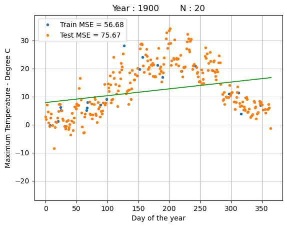
While linear regression is simple and interpretable, it struggles with the non-linear dependency between the day of the year and the temperature.
Instead, we can fit polynomial models of increasing degree \(n\) to better fit the temperature.
where \(x\) is the day of the year and \(w_i\) are the coefficients of the polynomial.
The trick is that we can represent the polynomial regression as a linear regression in a higher-dimensional space, where we replace the original feature \(x\) with a transformed vector \(\boldsymbol{\phi} (x)\) that contains the polynomial features \(x^0\), \(x^1, x^2, \dots, x^n\) as entries.
Given this vector, we can write the polynomial regression as a linear regression in the transformed space, where the polynomial coefficients are the weights of the linear regression:
Here is a simple implementation of the polynomial feature transformation:
def polynomial_transform(x, degree=2):
    """
    Transform the input data into polynomial features of a specified degree.
    Args:
        x (numpy.ndarray): Input data of shape (N, 1) where N is the number of samples.
        degree (int): Degree of the polynomial features.
    Returns:
        numpy.ndarray: Transformed data of shape (N, degree) containing polynomial features.
    """
    phi_polynomial = np.empty((x.shape[0], degree+1))
    for i in range(degree+1):
        phi_polynomial[:, i] = x[:, 0] ** (i)
    return phi_polynomial
While we do not yet have all the tools to find the optimal weight vector \(\bf{w}\), we can already look at the results of using linear regression with this transformed vector to predict the temperature.
Show code cell source
class RidgeRegression:
    """
    Ridge Regression model.

    Attributes:
        ridge (float): Regularization parameter.
        N (int): Number of samples.
        w (numpy.ndarray): Coefficients of the fitted model.
        fit_mean (bool): Whether to fit the mean of the data.
    """
    def __init__(self, ridge=0.0, fit_mean=False):
        """
        Initializes the KernelRidgeRegression model with specified parameters.

        Args:
            ridge (float, optional): Regularization parameter. Defaults to 0.0.
            fit_mean (bool, optional): Whether to fit the mean of the data. Defaults to False.
        """
        self.ridge = ridge
        self.N = None
        self.w = None
        self.fit_mean = fit_mean

    def fit(self, X, y):
        """
        Fits the model to the training data.

        Args:
            X (numpy.ndarray): Training feature design matrix.
            y (numpy.ndarray): Target variable.

        Notes:
            The method computes the coefficients of the model using the provided kernel matrix and target variable.
        """
        if self.fit_mean:
            self.mean_y = y.mean(0)
            self.mean_X = X.mean(0)
            X = X - self.mean_X[np.newaxis,:]
            y = y - self.mean_y
        else:
            self.mean_y = 0.0
        self.N = X.shape[0]
        XX = X.T @ X + np.eye(X.shape[1]) * self.ridge
        Xy = X.T @ y
        self.w = np.linalg.lstsq(XX, Xy, rcond=None)[0]

    def pred(self, X_star):
        """
        Predicts target variable for new data.

        Args:
            X_star (numpy.ndarray): Feature design matrix for new data.

        Returns:
            numpy.ndarray: Predicted target variable.
        """
        if self.fit_mean:
            X_star = X_star - self.mean_X[np.newaxis,:]
        return X_star @ self.w + self.mean_y

    def mse(self, X, y):
        """
        Computes mean squared error.

        Args:
            X (numpy.ndarray): Feature design matrix.
            y (numpy.ndarray): Target variable.

        Returns:
            float: Mean squared error.
        """
        y_pred = self.pred(X)
        residual = y - y_pred
        return np.mean(residual * residual)

    def score(self, X, y):
        """
        Computes the score of the model.

        Args:
            X (numpy.ndarray): Feature design matrix.
            y (numpy.ndarray): Target variable.

        Returns:
            float: Score of the model.
        """
        return self.mse(X=X, y=y)

def fit_polynomial(degree = 2):
    fit_mean = False     # fit a separate mean for y in the linear regression?
    ridge = 0     # strength of the L2 penalty in ridge regression

    x_train = data_train.days.values[:N_train][:,np.newaxis] * 1.0
    X_train = polynomial_transform(x_train, degree=degree)
    y_train = data_train.TMAX.values[:N_train]

    reg = RidgeRegression(fit_mean=fit_mean, ridge=ridge)
    reg.fit(X_train, y_train)

    x_days = np.arange(366)[:,np.newaxis]
    X_days = polynomial_transform(x_days, degree=degree)
    y_days_pred = reg.pred(X_days)

    x_test = data_test.days.values[:,np.newaxis] * 1.0
    X_test = polynomial_transform(x_test, degree=degree)
    y_test = data_test.TMAX.values
    y_test_pred = reg.pred(X_test)
    # print("training MSE : %.4f" % reg.mse(X_train, y_train))
    # print("test MSE     : %.4f" % reg.mse(X_test, y_test))

    fig = plt.figure()
    ax = plt.plot(x_train,y_train,'.')
    ax = plt.plot(x_test,y_test,'.')
    ax = plt.legend(["train MSE = %.2f" % reg.mse(X_train, y_train),"test MSE = %.2f" % reg.mse(X_test, y_test)])
    ax = plt.plot(x_days,y_days_pred)
    ax = plt.ylim([-27,39])
    ax = plt.xlabel("day of the year")
    ax = plt.ylabel("Maximum Temperature - degree C")
    ax = plt.title("Polynomial of degree %i    Year : %i        N : %i" % (degree, YEAR, N_train))
# fit_polynomial(degree=2)
fit_polynomial(degree=3)
# fit_polynomial(degree=4)
fit_polynomial(degree=7)
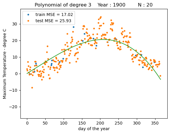
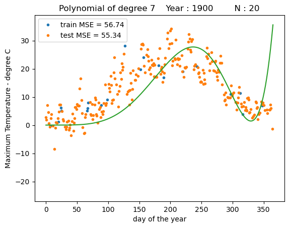
We can see that a polynomial regression models with higher order polynomials can fit the data much better than a linear regression model, but also at some point may provide unrealisticly high predictions towards the end of the year.