Clustering

Clustering is an unsupervised learning task where the goal is to discover meaningful groups, or “clusters,” within unlabeled data. Unlike supervised methods (classification and regression), clustering algorithms rely solely on the inherent structure of data points, without any explicit labels or target values.

Formally, clustering involves:

• Data: A set of unlabeled points typically represented as vectors in a vector space:

\[ \mathbf{x} \in \mathbb{R}^n \]

• Objective: Partition the data into distinct groups (clusters) such that points within the same cluster are more similar to each other than to points in different clusters.

Let’s look at an example of clustering in action.

Show code cell source Hide code cell source

import numpy as np
import matplotlib.pyplot as plt

np.random.seed(0) 
n=50 # samples per c1uster
centers= [ [3,4], [8,3], [2,10], [9,9], ]
dataset=np.zeros((0,3))
sigmas = [ 0.5, 1, 1.5, 2 ]

# Generate clusters
for i in range(len(centers)):
    correlation=(np.random.rand()-0.5)*2
    center=centers[i]
    sigma=sigmas[i]
    cluster=np.random.multivariate_normal(center, [[sigma, correlation],[correlation, sigma]], n)
    label=np.zeros((n,1))+i
    cluster=np.hstack([cluster,label])
    dataset=np.vstack([dataset,cluster])

class KMeans:
    def __init__(self, n_clusters=3):
        self.n_clusters = n_clusters

    def fit(self, X, num_iterations=10):
        # Randomly initialize cluster centers
        self.centers = X[np.random.choice(X.shape[0], self.n_clusters, replace=False)]
        self.labels = np.zeros(X.shape[0])

        for _ in range(num_iterations):  # Iterate a fixed number of times
            old_labels = self.labels.copy()
            self.iterate(X)
            # Check for convergence (optional)
            if np.all(self.labels == old_labels):
                break

    def iterate(self, X):
        # Assign clusters based on closest center
        distances = np.linalg.norm(X[:, np.newaxis] - self.centers, axis=2)
        self.labels = np.argmin(distances, axis=1)

        # Update cluster centers
        for i in range(self.n_clusters):
            self.centers[i] = X[self.labels == i].mean(axis=0)
    
    def predict(self, X):
        distances = np.linalg.norm(X[:, np.newaxis] - self.centers, axis=2)
        return np.argmin(distances, axis=1)

kmeans = KMeans(n_clusters=4)
kmeans.fit(dataset[:,:2], num_iterations=0)
plt.figure(figsize=(5,5))
ax = plt.scatter(kmeans.centers[:,0], kmeans.centers[:,1], c='red', s=200, alpha=0.5)
ax = plt.scatter(dataset[:,0], dataset[:,1], c=dataset[:,2], s=100, alpha=0.5)
ax = plt.title("Generated Dataset with Random Cluster Centers")

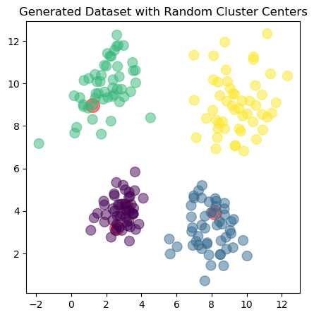
The dataset consists of four clusters, each represented by a different color. The goal of clustering is to identify these groups based on the data points’ proximity in the feature space. We will use the \(k\)-means algorithm to achieve this. The red dots in the plot represent the initial cluster centers, which are randomly selected from the dataset.

The k-means algorithm is a popular clustering method that partitions data into \(k\) clusters by iteratively refining the cluster centers until convergence, effectively grouping similar data points together. It does this by iteratively assigning points to the nearest cluster center and updating the centers based on the mean of the assigned points.

Show code cell source Hide code cell source

for i in range(6):
    kmeans.iterate(dataset[:,:2])
    plt.figure(figsize=(5,5))
    ax = plt.scatter(kmeans.centers[:,0], kmeans.centers[:,1], c='red', s=200, alpha=0.5)
    ax = plt.scatter(dataset[:,0], dataset[:,1], c=kmeans.predict(dataset[:,:2]), s=100, alpha=0.5)
    ax = plt.title("KMeans Clustering after {} iterations".format(i+1))

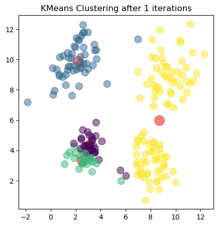
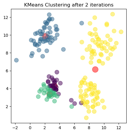
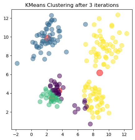
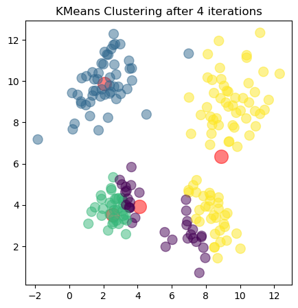
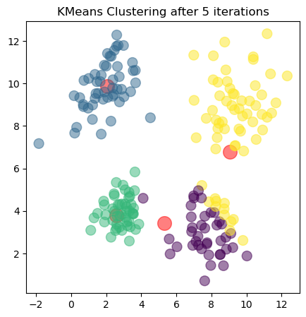
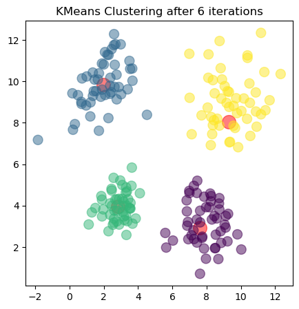
The plots show the updated cluster centers (red dots) and the data points colored according to their assigned clusters for each iteration. As the algorithm iterates, the cluster centers move closer to the actual centers of the clusters in the dataset, demonstrating how clustering algorithms can effectively uncover underlying patterns in unlabeled data.

Examples of clustering tasks

• Customer Segmentation: Grouping customers based on purchasing behavior to tailor marketing strategies.

• Image Segmentation: Dividing an image into regions with similar colors or textures, often used in computer vision tasks.

• Document Clustering: Organizing documents into topics or themes based on content similarity, useful in information retrieval and natural language processing.

• Anomaly Detection: Identifying unusual patterns or outliers in data, such as fraud detection in financial transactions.

• Genomic Data Analysis: Grouping genes or proteins based on expression patterns, aiding in biological research and drug discovery.

• Social Network Analysis: Identifying communities or groups within social networks based on user interactions or relationships.

Geometric intuition

Clustering algorithms often use distance-based metrics to determine similarity between data points, making metrics, norms, and vector spaces fundamental concepts. Clusters typically emerge as regions of feature space with high density or proximity of data points.

One common geometric interpretation of clustering is identifying regions separated by boundaries of low density or large distances, capturing the natural grouping inherent in data distributions.

Common clustering algorithms

• \(k\)-Means Clustering: Iteratively assigns data points to the nearest centroid (cluster center) based on Euclidean distance, showcasing fundamental vector space concepts and optimization procedures.

• DBSCAN (Density-Based Spatial Clustering): Identifies clusters based on local point density, explicitly using distance metrics to define dense regions.

• Spectral Clustering: Utilizes eigenvector decompositions of graph-based representations of the data, connecting directly to linear algebra and matrix factorization methods.

• Gaussian Mixture Models (GMM): Models data as a mixture of multiple Gaussian distributions, leveraging probabilistic frameworks and distance metrics to define clusters.

Clustering in this book

In this book, clustering serves as a motivating example to introduce and reinforce concepts in linear algebra. You’ll explore how distances between points are defined in metric spaces, understand cluster structure through norms and inner product spaces, and learn how advanced matrix decompositions (such as eigen-decompositions and singular value decomposition) enable effective clustering algorithms.

Through these examples, you’ll develop a deeper understanding of how mathematical foundations shape clustering methods and discover powerful tools for uncovering structure in complex, unlabeled datasets.