Inner product spaces#
Inner product spaces allow us to generalize ideas of angles, lengths, and orthogonality beyond traditional Euclidean geometry. They are foundational in machine learning algorithms involving geometric intuition, similarity measurement, and projection methods.
An inner product on a real vector space \(V\) is a function \(\langle \cdot, \cdot \rangle : V \times V \to \mathbb{R}\) satisfying
(i) \(\langle \mathbf{x}, \mathbf{x} \rangle \geq 0\), with equality if and only if \(\mathbf{x} = \mathbf{0}\)
(ii) \(\langle \alpha\mathbf{x} + \beta\mathbf{y}, \mathbf{z} \rangle = \alpha\langle \mathbf{x}, \mathbf{z} \rangle + \beta\langle \mathbf{y}, \mathbf{z} \rangle\)
(iii) \(\langle \mathbf{x}, \mathbf{y} \rangle = \langle \mathbf{y}, \mathbf{x} \rangle\)
for all \(\mathbf{x}, \mathbf{y}, \mathbf{z} \in V\) and all \(\alpha,\beta \in \mathbb{R}\).
A vector space endowed with an inner product is called an inner product space.
Note that any inner product on \(V\) induces a norm on \(V\):
One can verify that the axioms for norms are satisfied under this definition and follow (almost) directly from the axioms for inner products. Therefore any inner product space is also a normed space (and hence also a metric space).
Two vectors \(\mathbf{x}\) and \(\mathbf{y}\) are said to be orthogonal if \(\langle \mathbf{x}, \mathbf{y} \rangle = 0\); we write \(\mathbf{x} \perp \mathbf{y}\) for shorthand. Orthogonality generalizes the notion of perpendicularity from Euclidean space. If two orthogonal vectors \(\mathbf{x}\) and \(\mathbf{y}\) additionally have unit length (i.e. \(\|\mathbf{x}\| = \|\mathbf{y}\| = 1\)), then they are described as orthonormal.
The standard inner product on \(\mathbb{R}^n\) is given by
The matrix notation on the righthand side (see the Transposition section if it’s unfamiliar) arises because this inner product is a special case of matrix multiplication where we regard the resulting \(1 \times 1\) matrix as a scalar. The inner product on \(\mathbb{R}^n\) is also often written \(\mathbf{x}\cdot\mathbf{y}\) (hence the alternate name dot product). The two-norm \(\|\cdot\|_2\) on \(\mathbb{R}^n\) is induced by this inner product.
The inner product on \(\mathbb{R}^n\) induces the length (or two-norm) on \(\mathbb{R}^n\):
This is the familiar Euclidean length of a vector in \(\mathbb{R}^n\).
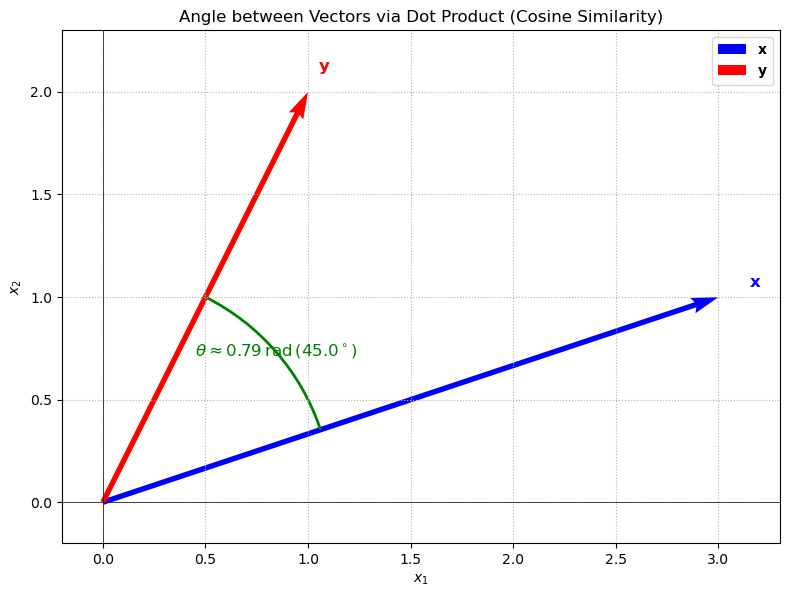
The inner product on \(\mathbb{R}^n\) induces the following angle between two vectors \(\mathbf{x}\) and \(\mathbf{y}\):
This angle is well-defined as long as \(\mathbf{x}\) and \(\mathbf{y}\) are not both the zero vector. The angle is \(0\) if \(\mathbf{x}\) and \(\mathbf{y}\) are parallel (i.e. \(\mathbf{x} = t\mathbf{y}\) for some \(t \in \mathbb{R}\)), and \(\pi/2\) if they are orthogonal. The cosine of the angle is given by the cosine similarity between \(\mathbf{x}\) and \(\mathbf{y}\):
This is a common measure of similarity between two vectors, and is often used in machine learning applications.
Show code cell source
import numpy as np
import matplotlib.pyplot as plt
from matplotlib.patches import Arc

# Define two non-zero vectors in R^2.
x = np.array([3, 1])
y = np.array([1, 2])

# Compute inner products and norms.
dot_xy = np.dot(x, y)
norm_x = np.linalg.norm(x)
norm_y = np.linalg.norm(y)

# Compute cosine similarity and angle theta (in radians).
cos_theta = dot_xy / (norm_x * norm_y)
theta = np.arccos(cos_theta)  # angle between x and y, in radians
theta_deg = np.degrees(theta)

# Compute the polar angles of vectors x and y (in degrees)
angle_x = np.degrees(np.arctan2(x[1], x[0]))
angle_y = np.degrees(np.arctan2(y[1], y[0]))

# Ensure the arc goes in the correct direction:
# If angle_y is less than angle_x, we add 360 to angle_y.
if angle_y < angle_x:
    angle_y += 360

# Choose a radius for the arc (e.g. half the minimum norm)
arc_radius = min(norm_x, norm_y) / 2

# Create the arc patch from angle_x to angle_y.
arc = Arc((0, 0), 2*arc_radius, 2*arc_radius, angle=0,
          theta1=angle_x, theta2=angle_y, color='green', lw=2)

# Set up the plot.
plt.figure(figsize=(8, 8))
ax = plt.gca()

# Plot vector x and vector y, both originating at (0, 0).
origin = np.array([0, 0])
ax.quiver(*origin, *x, angles='xy', scale_units='xy', scale=1, color='blue', label=r"$\mathbf{x}$")
ax.quiver(*origin, *y, angles='xy', scale_units='xy', scale=1, color='red', label=r"$\mathbf{y}$")
ax.text(x[0]*1.05, x[1]*1.05, r"$\mathbf{x}$", color='blue', fontsize=12)
ax.text(y[0]*1.05, y[1]*1.05, r"$\mathbf{y}$", color='red', fontsize=12)

# Add the arc representing the angle between x and y.
ax.add_patch(arc)

# Compute the midpoint of the arc (in degrees and then convert to radians)
arc_mid_angle = (angle_x + angle_y) / 2.0
arc_mid_rad = np.radians(arc_mid_angle)
arc_text_x = arc_radius * np.cos(arc_mid_rad)
arc_text_y = arc_radius * np.sin(arc_mid_rad)

# Annotate the arc with the angle value (in radians).
ax.text(arc_text_x, arc_text_y,
        f"$\\theta\\approx {theta:.2f}\\,\\text{{rad}}\\,({theta_deg:.1f}^\\circ)$",
        color='green', fontsize=12, ha='center', va='center')

# Add axis labels, title, grid, and legend.
plt.xlabel("$x_1$")
plt.ylabel("$x_2$")
plt.title("Angle between Vectors via Dot Product (Cosine Similarity)")
plt.axhline(0, color='black', linewidth=0.5)
plt.axvline(0, color='black', linewidth=0.5)
plt.xlim(-0.2, max(x[0], y[0]) + 0.3)
plt.ylim(-0.2, max(x[1], y[1]) + 0.3)
plt.legend(loc='upper right')
plt.gca().set_aspect('equal', adjustable='box')
plt.grid(True, linestyle=':')
plt.tight_layout()
plt.show()
Pythagorean Theorem#
The well-known Pythagorean theorem generalizes naturally to arbitrary inner product spaces.
Theorem (Pythagorean theorem)
If \(\mathbf{x} \perp \mathbf{y}\), then
Proof. Suppose \(\mathbf{x} \perp \mathbf{y}\), i.e. \(\langle \mathbf{x}, \mathbf{y} \rangle = 0\). Then
as claimed. ◻
Show code cell source
import numpy as np
import matplotlib.pyplot as plt

# Define two perpendicular vectors x and y.
x = np.array([3, 0])
y = np.array([0, 4])
sum_xy = x + y

# Compute the norms (Euclidean norm)
norm_x = np.linalg.norm(x)
norm_y = np.linalg.norm(y)
norm_sum = np.linalg.norm(sum_xy)

# Verify the Pythagorean theorem numerically
lhs = norm_sum**2
rhs = norm_x**2 + norm_y**2

# Set up the plot
plt.figure(figsize=(8, 8))
origin = np.array([0, 0])

# Plot vector x, y, and x+y
plt.quiver(*origin, *x, angles='xy', scale_units='xy', scale=1, color='blue', label=r"$\mathbf{x}$")
plt.quiver(*origin, *y, angles='xy', scale_units='xy', scale=1, color='green', label=r"$\mathbf{y}$")
plt.quiver(*origin, *sum_xy, angles='xy', scale_units='xy', scale=1, color='red', label=r"$\mathbf{x}+\mathbf{y}$")

# Mark the right angle at the origin
plt.plot([x[0], x[0]], [0, y[1]], 'k--', linewidth=1)

# Annotate the plot with norm values
plt.text(x[0]/2, x[1]-0.3, f"{norm_x:.1f}", color='blue', fontsize=12)
plt.text(y[0]-1.0, y[1]/2, f"{norm_y:.1f}", color='green', fontsize=12)
plt.text(sum_xy[0]/2+0.2, sum_xy[1]/2+0.2, f"{norm_sum:.1f}", color='red', fontsize=12)

plt.xlabel("$x_1$")
plt.ylabel("$x_2$")
plt.title("Pythagorean Theorem in an Inner Product Space")
plt.xlim(-1, 4.3)
plt.ylim(-1, 4.3)
plt.grid(True, linestyle=':')
plt.legend()

# Print the numerical check in the console
print(f"||x+y||^2 = {lhs:.2f}")
print(f"||x||^2 + ||y||^2 = {rhs:.2f}")

plt.tight_layout()
plt.show()
||x+y||^2 = 25.00
||x||^2 + ||y||^2 = 25.00
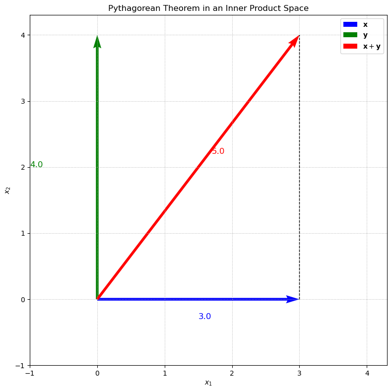
In this example, we choose two perpendicular vectors \(\mathbf{x}\) and \(\mathbf{y}\) (for instance, \(\mathbf{x}=(3, 0)\) and \(\mathbf{y}=(0, 4)\)) and plot these vectors along with their sum \(\mathbf{x}+\mathbf{y}\). The plot visually demonstrates the Pythagorean theorem, where the lengths of the sides of the right triangle formed by \(\mathbf{x}\) and \(\mathbf{y}\) correspond to their norms. The dashed line indicates the right angle between the two vectors.
Cauchy-Schwarz inequality#
The Cauchy-Schwarz inequality is a fundamental result in linear algebra and functional analysis. It states that the absolute value of the inner product of two vectors is less than or equal to the product of their norms. This inequality is a powerful tool in various fields, including machine learning, statistics, and optimization.
Theorem (Cauchy–Schwarz Inequality)
For all \(\mathbf{x}, \mathbf{y} \in V\),
with equality if and only if \(\mathbf{x}\) and \(\mathbf{y}\) are linearly dependent.
For a proof see the Appendix of the book.
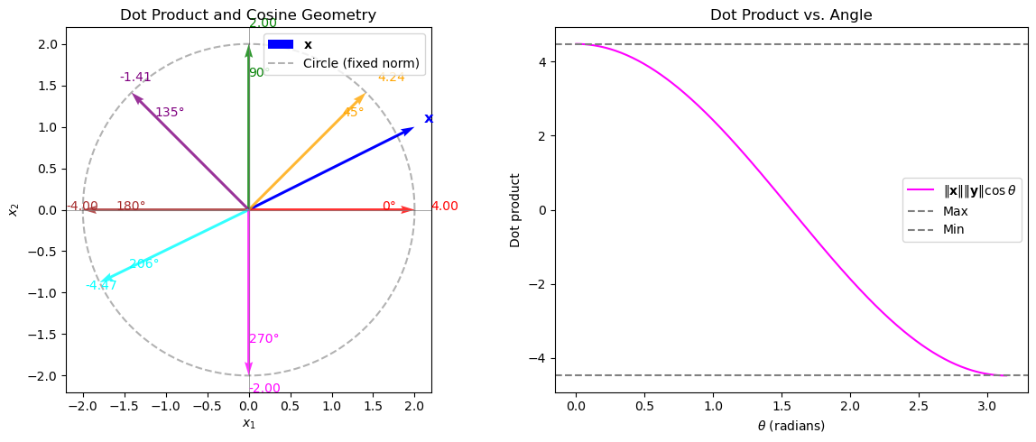
We attempt a visual explanation of the Cauchy–Schwarz inequality by relating the dot product to the cosine of the angle between vectors and illustrating its geometric implications for a linear classifier’s decision boundary. In this visualization, we fix a vector \(\mathbf{x}\) and draw several vectors \(\mathbf{y}\) on a circle (so that \(\|\mathbf{y}\|\) is fixed). For each such \(\mathbf{y}\), we annotate the computed dot product (which equals \(\|\mathbf{x}\|\|\mathbf{y}\|\cos\theta\)). In a separate subplot, we also plot the function \(f(\theta)=\|\mathbf{x}\|\|\mathbf{y}\|\cos\theta\) versus \(\theta\) to show that the dot product is maximized when \(\mathbf{y}\) is aligned with \(\mathbf{x}\) and minimized when it is opposite.
Show code cell source
import numpy as np
import matplotlib.pyplot as plt

# Define a fixed vector x.
x = np.array([2, 1])
norm_x = np.linalg.norm(x)

# Define a fixed norm for y.
norm_y = 2.0

# Create a figure with two subplots.
plt.figure(figsize=(12, 5))

# Subplot 1: Visualizing x and several y vectors.
plt.subplot(1, 2, 1)
plt.axhline(0, color='gray', linewidth=0.5)
plt.axvline(0, color='gray', linewidth=0.5)
plt.gca().set_aspect('equal')

# Plot vector x.
plt.quiver(0, 0, x[0], x[1], angles='xy', scale_units='xy', scale=1, color='blue', label=r"$\mathbf{x}$")
plt.text(x[0]*1.05, x[1]*1.05, r"$\mathbf{x}$", color='blue', fontsize=12)

# Define several angles for y (in radians).
angles_deg = [0, 45, 90, 135, 180, 206, 270]
thetas = np.deg2rad(angles_deg)
colors = ['red', 'orange', 'green', 'purple', 'brown', 'cyan', 'magenta']

# Plot a circle for reference (all y with fixed norm).
theta_circle = np.linspace(0, 2*np.pi, 300)
circle_x = norm_y * np.cos(theta_circle)
circle_y = norm_y * np.sin(theta_circle)
plt.plot(circle_x, circle_y, 'k--', alpha=0.3, label="Circle (fixed norm)")

# Plot vectors y at the specified angles and annotate their dot product.
for theta, c, deg in zip(thetas, colors, angles_deg):
    y = norm_y * np.array([np.cos(theta), np.sin(theta)])
    plt.quiver(0, 0, y[0], y[1], angles='xy', scale_units='xy', scale=1, color=c, alpha=0.8)
    dp = np.dot(x, y)
    # Place the annotation near the end of y.
    plt.text(y[0]*1.1, y[1]*1.1, f"{dp:.2f}", color=c, fontsize=10)
    plt.text(y[0]*0.8, y[1]*0.8, f"{deg}°", color=c, fontsize=10)

plt.title("Dot Product and Cosine Geometry")
plt.xlabel(r"$x_1$")
plt.ylabel(r"$x_2$")
plt.legend(loc="upper right")

# Subplot 2: Plot the dot product as a function of the angle between x and y.
plt.subplot(1, 2, 2)
theta_vals = np.linspace(0, np.pi, 300)
dp_vals = norm_x * norm_y * np.cos(theta_vals)
plt.plot(theta_vals, dp_vals, label=r"$\|\mathbf{x}\|\|\mathbf{y}\|\cos\theta$", color='magenta')
plt.axhline(norm_x * norm_y, color='gray', linestyle='--', label="Max")
plt.axhline(-norm_x * norm_y, color='gray', linestyle='--', label="Min")
plt.xlabel(r"$\theta$ (radians)")
plt.ylabel("Dot product")
plt.title("Dot Product vs. Angle")
plt.legend()

plt.tight_layout()
plt.show()
Explanation#
Subplot 1 (Geometry in \(\mathbb{R}^2\)):
The blue arrow represents the fixed vector \(\mathbf{x}\). The red, orange, green, purple, and brown arrows are various vectors \(\mathbf{y}\) on the circle of radius \(2\) (i.e. with fixed norm \(\|\mathbf{y}\| = 2\)) at angles \(0^\circ\), \(45^\circ\), \(90^\circ\), \(135^\circ\), and \(180^\circ\), respectively. For each \(\mathbf{y}\), the dot product \(\langle \mathbf{x}, \mathbf{y} \rangle\) is calculated and annotated. This illustrates that the dot product depends on the cosine of the angle between \(\mathbf{x}\) and \(\mathbf{y}\).Subplot 2 (Function Plot):
This subplot shows the function \(f(\theta) = \|\mathbf{x}\|\|\mathbf{y}\|\cos\theta\) as a function of the angle \(\theta\). The maximum and minimum possible dot products occur when \(\theta=0\) or \(\theta=\pi\), corresponding to perfect alignment and opposite direction, respectively. This visualization reinforces the concept that the dot product is essentially \(\|\mathbf{x}\|\|\mathbf{y}\|\cos\theta\).
Kernels as Generalized Inner Products#
The notion of inner product spaces provides a powerful generalization called kernels, leading to the idea of kernel methods in machine learning. Kernels allow us to implicitly map data into high-dimensional spaces where classification or regression tasks become simpler.
A kernel function \(k(\mathbf{x}, \mathbf{y})\) is defined as:
where:
\(\phi(\mathbf{x})\) is a feature mapping from the original feature space into a possibly high-dimensional (or even infinite-dimensional) inner product space.
This new space is called a Reproducing Kernel Hilbert Space (RKHS).
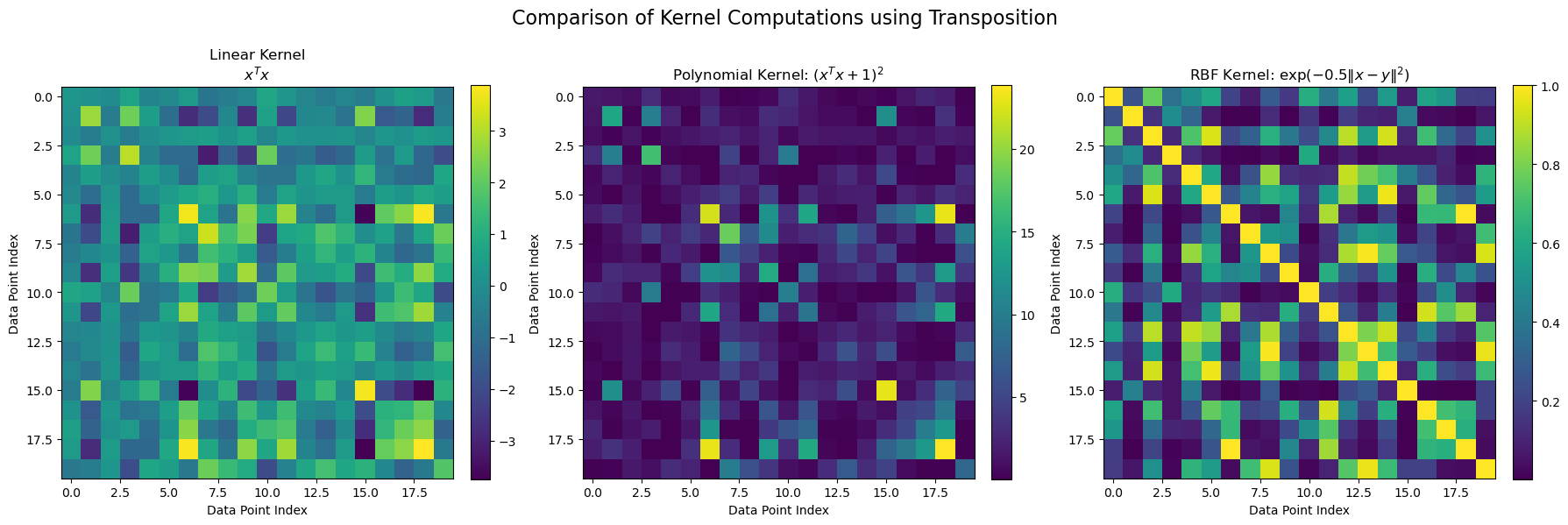
Common kernels include:
The linear kernel \(k_{\mathrm{linear}}(\mathbf{x},\mathbf{y}) = \mathbf{x}^{\!\top}\mathbf{y}\),
The polynomial kernel \(k_{\mathrm{poly}}(\mathbf{x},\mathbf{y}) = (\mathbf{x}^{\!\top}\mathbf{y} + c)^d\), and
The Gaussian (RBF) kernel \(k_{\mathrm{RBF}}(\mathbf{x},\mathbf{y}) = \exp(-\gamma\|\mathbf{x}-\mathbf{y}\|^2)\).
Show code cell source
import numpy as np
import matplotlib.pyplot as plt

def linear_kernel(X):
    """
    Compute the linear (dot product) kernel matrix.
    For a data matrix X (shape: [n_samples, n_features]), the linear kernel is:
      k_linear(x, y) = x^T y.
    """
    return X @ X.T

def polynomial_kernel(X, c=1.0, d=2):
    """
    Compute the polynomial kernel matrix.

    k_poly(x,y) = (x^T y + c)^d.
    """
    K_lin = X @ X.T
    return (K_lin + c) ** d

def rbf_kernel(X, gamma=0.5):
    """
    Compute the Gaussian (RBF) kernel matrix.

    k_RBF(x,y) = exp(-gamma ||x - y||^2).
    """
    # Compute squared Euclidean norms for each data point.
    sq_norms = np.sum(X**2, axis=1)
    # Compute the squared distance matrix using broadcasting:
    D = sq_norms.reshape(-1, 1) - 2 * X @ X.T + sq_norms.reshape(1, -1)
    return np.exp(-gamma * D)

# Generate a synthetic dataset in R^n (here, n=2) with m data points.
np.random.seed(42)
m, n = 20, 2  # 20 data points in 2D
X = np.random.randn(m, n)

# Compute kernel matrices.
K_linear = linear_kernel(X)
K_poly = polynomial_kernel(X, c=1.0, d=2)
K_rbf = rbf_kernel(X, gamma=0.5)

# Create subplots for the three kernels.
fig, axs = plt.subplots(1, 3, figsize=(18, 6))

# Plot the linear (dot product) kernel matrix.
im0 = axs[0].imshow(K_linear, cmap='viridis', aspect='equal')
axs[0].set_title("Linear Kernel\n$x^Tx$")
axs[0].set_xlabel("Data Point Index")
axs[0].set_ylabel("Data Point Index")
plt.colorbar(im0, ax=axs[0], fraction=0.046, pad=0.04)

# Plot the polynomial kernel matrix.
im1 = axs[1].imshow(K_poly, cmap='viridis', aspect='equal')
axs[1].set_title(r"Polynomial Kernel: $(x^Tx + 1)^2$")
axs[1].set_xlabel("Data Point Index")
axs[1].set_ylabel("Data Point Index")
plt.colorbar(im1, ax=axs[1], fraction=0.046, pad=0.04)

# Plot the Gaussian (RBF) kernel matrix.
im2 = axs[2].imshow(K_rbf, cmap='viridis', aspect='equal')
axs[2].set_title(r"RBF Kernel: $\exp(-0.5\|x-y\|^2)$")
axs[2].set_xlabel("Data Point Index")
axs[2].set_ylabel("Data Point Index")
plt.colorbar(im2, ax=axs[2], fraction=0.046, pad=0.04)

plt.suptitle("Comparison of Kernel Computations using Transposition", fontsize=16)
plt.tight_layout(rect=[0, 0.03, 1, 0.95])
plt.show()
Kernelized Nearest Centroid Classifier:#
We have already learned that we can obtain a non-linear version of a linear classifier such as the nearest centroid classifier by using non-linear basis functions \(\phi(\cdot)\) to map the data into a higher-dimensional space.
where \(\phi_i(\cdot)\) are real-valued basis functions.
The nearest centroid classifier assigns a new point \(\mathbf{x}\) to the class \(k\) whose centroid \(\mathbf{c}_k\) is closest to \(\phi(\mathbf{x})\). The centroid \(\mathbf{c}_k\) is computed as the mean of the training points in class \(k\) after applying the mapping \(\phi\):
where \(N_k\) is the number of training examples in class \(k\).
Instead of explicitly computing the centroid in the original space, we can implicitly compute distances in a high-dimensional space using inner products and their implied distance metric only.
The distance between a point \(\phi(\mathbf{x})\) and the centroid \(\mathbf{c}_k\) can be expressed in terms of the inner products involving \(\phi(\mathbf{x})\) and \(\mathbf{c}_k\):
Using the defitintion of the kernel function \(k(\mathbf{x},\mathbf{y})=\langle\phi(\mathbf{x}, \phi(\mathbf{y}))\) and the fact that \(\mathbf{c}_k\) is the average of all the training data points in class \(k\), we can express this distance only based on kernels between \(\mathbf{x}\) and the training points in class \(k\):
Using this kernelized distance, the classifier assigns \(\mathbf{x}\) to the class \(k\) for which \(\|\phi(\mathbf{x}) - \mathbf{c}_k\|^2\) is minimal. In this way, the kernelized nearest centroid classifier operates solely via inner products—thus allowing the algorithm to implicitly work in high-dimensional feature spaces without ever computing the mapping \(\phi\) explicitly. This is particularly useful when the mapping is computationally expensive or infeasible to compute directly due to its high (or even infinite) dimensionality. Thus, a kernelized nearest centroid classifier can classify points using arbitrary inner product spaces defined by kernels, allowing the classifier to handle complex, nonlinear patterns in the data.
import numpy as np

class KernelNearestCentroid:
    def __init__(self, kernel=None):
        """
        Initialize the Kernelized Nearest Centroid Classifier.

        Parameters:
        -----------
        kernel : function or None
            A function that takes two vectors and returns a scalar,
            representing the inner product in the feature space.
            If None, a default RBF kernel with sigma=1.0 is used.
        """
        if kernel is None:
            # Default: RBF kernel with sigma=1.0 (gamma=1/(2*sigma^2)=0.5)
            self.kernel = lambda x, y: np.exp(-np.linalg.norm(x - y)**2 / 2.0)
        else:
            self.kernel = kernel
        self.classes_ = None
        self.class_indices_ = {}  # mapping from class to indices in training set
        self.N_k_ = {}            # number of training examples per class
        self.K_train_ = None      # kernel matrix for training data
        self.K_centroid_sqr_ = {} # precomputed term: (1/N_k^2)*sum_{i,j in class k} k(x_i, x_j)
        self.X_train_ = None
        self.y_train_ = None

    def fit(self, X, y):
        """
        Fit the kernelized nearest centroid classifier.

        Parameters:
        -----------
        X : array-like, shape (n_samples, n_features)
            Training data.
        y : array-like, shape (n_samples,)
            Class labels.
        """
        self.X_train_ = np.asarray(X)
        self.y_train_ = np.asarray(y)
        self.classes_ = np.unique(self.y_train_)
        n = self.X_train_.shape[0]
        # Precompute kernel matrix on training data
        self.K_train_ = np.zeros((n, n))
        for i in range(n):
            for j in range(i, n):
                k_val = self.kernel(self.X_train_[i], self.X_train_[j])
                self.K_train_[i, j] = k_val
                self.K_train_[j, i] = k_val

        # For each class, store indices and precompute centroid norm squared in feature space
        for cls in self.classes_:
            indices = np.where(self.y_train_ == cls)[0]
            self.class_indices_[cls] = indices
            N_k = len(indices)
            self.N_k_[cls] = N_k
            # Compute the double-sum term for class centroid: (1/N_k^2)*sum_{i,j in class} k(x_i, x_j)
            K_cls = self.K_train_[np.ix_(indices, indices)]
            self.K_centroid_sqr_[cls] = np.sum(K_cls) / (N_k**2)

    def decision_function(self, x):
        """
        Compute the squared distance in feature space from x to each class centroid.
        The kernelized squared distance for class k is given by:

            d^2(x, c_k) = k(x, x)
                          - (2/N_k)*sum_{i:y_i=k} k(x, x_i)
                          + (1/N_k^2)*sum_{i,j:y_i,y_j=k} k(x_i,x_j)

        Returns:
        --------
        distances : dict
            Dictionary mapping class label to the computed squared distance.
        """
        distances = {}
        k_xx = self.kernel(x, x)
        for cls in self.classes_:
            indices = self.class_indices_[cls]
            N_k = self.N_k_[cls]
            # Compute sum_{i in class} k(x, x_i)
            k_x_class = np.array([self.kernel(x, self.X_train_[i]) for i in indices])
            term2 = (2.0 / N_k) * np.sum(k_x_class)
            term3 = self.K_centroid_sqr_[cls]
            distances[cls] = k_xx - term2 + term3
        return distances

    def predict(self, X):
        """
        Predict the class labels for the given set of data.

        Parameters:
        -----------
        X : array-like, shape (n_samples, n_features)

        Returns:
        --------
        y_pred : ndarray, shape (n_samples,)
            Predicted class labels.
        """
        X = np.asarray(X)
        preds = []
        for x in X:
            distances = self.decision_function(x)
            pred = min(distances, key=distances.get)
            preds.append(pred)
        return np.array(preds)
Show code cell source
import matplotlib.pyplot as plt
# -------------------------------
# Demonstration on Synthetic Data
# -------------------------------
if __name__ == "__main__":
    # Generate synthetic 2D data for two classes
    np.random.seed(42)
    X_class0 = np.random.randn(20, 2) + np.array([1, 1])
    X_class1 = np.random.randn(20, 2) + np.array([-1, -1])
    X_train = np.vstack((X_class0, X_class1))
    y_train = np.array([0]*20 + [1]*20)

    # Instantiate and fit the classifier with an RBF kernel
    clf = KernelNearestCentroid(kernel=lambda x, y: np.exp(-np.linalg.norm(x - y)**2 / 2.0))
    clf.fit(X_train, y_train)

    # Create a grid for visualizing the decision boundary
    xx, yy = np.meshgrid(np.linspace(-4, 4, 300), np.linspace(-4, 4, 300))
    grid = np.c_[xx.ravel(), yy.ravel()]
    Z = clf.predict(grid)
    Z = Z.reshape(xx.shape)

    # Plot decision regions and training data
    plt.figure(figsize=(8, 6))
    plt.contourf(xx, yy, Z, alpha=0.3, cmap=plt.cm.coolwarm)
    plt.scatter(X_train[y_train==0][:, 0], X_train[y_train==0][:, 1],
                color='blue', label='Class 0', edgecolor='k')
    plt.scatter(X_train[y_train==1][:, 0], X_train[y_train==1][:, 1],
                color='red', label='Class 1', edgecolor='k')
    plt.title("Kernelized Nearest Centroid Classifier")
    plt.xlabel("x1")
    plt.ylabel("x2")
    plt.legend()
    plt.grid(True, linestyle=":")
    plt.tight_layout()
    plt.show()
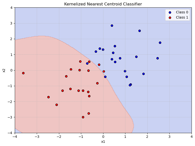
Insights:#
Inner products provide a flexible geometric tool for measuring angles and similarity.
Kernels use inner products implicitly to map data into spaces where classification is simplified.
The kernelized nearest centroid classifier offers a straightforward way to appreciate how inner product spaces generalize standard linear classifiers, enhancing their expressive power in practical ML scenarios.
This approach naturally motivates the importance of inner product spaces and kernels in machine learning.