Representation Learning

Representation learning (also known as feature learning or dimensionality reduction) is an unsupervised learning task aimed at discovering efficient, meaningful, and compact representations of data. High-dimensional data often contain redundancy, noise, or irrelevant information, making it computationally expensive and challenging to analyze or visualize directly. Representation learning addresses this by embedding the data into lower-dimensional spaces that retain its essential structure and properties.

Formally, representation learning involves:

• Data: Unlabeled data points represented in a high-dimensional vector space:

\[ \mathbf{x} \in \mathbb{R}^n \quad (n \text{ is large}) \]

• Objective: Find a mapping (f) that transforms the data to a lower-dimensional representation, preserving as much relevant information as possible:

\[ f : \mathbb{R}^n \rightarrow \mathbb{R}^d, \quad \text{where } d \ll n \]

Geometric intuition

Representation learning can be thought of as finding simplified geometric structures within complex, high-dimensional spaces. Methods such as Principal Component Analysis (PCA) explicitly seek low-dimensional subspaces that capture the directions of maximum variance in data. By projecting onto these subspaces, the data becomes easier to visualize, analyze, and use for subsequent tasks like clustering, classification, or regression.

Common representation learning methods

• Principal Component Analysis (PCA): A linear dimensionality reduction method that projects data onto directions (principal components) of maximal variance, relying heavily on linear algebra concepts like eigen-decompositions and the singular value decomposition (SVD).

• Kernel PCA: A nonlinear extension of PCA that uses kernel functions and inner product spaces to capture complex data structures.

• Autoencoders: Neural network-based methods that learn nonlinear, compressed representations by reconstructing input data, leveraging optimization and linear algebra.

• Probabilistic PCA and Factor Analysis: Methods that use probabilistic modeling and linear algebra to learn low-dimensional representations while quantifying uncertainty in dimensionality reduction.

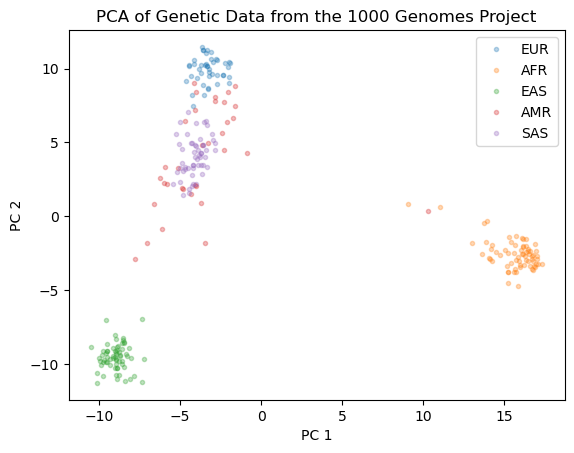
Principal Components Analysis of Genetic Data

In the example below, we will use the Principal Component Analysis (PCA) algorithm to reduce the dimensionality of a genetic dataset from the 1000 genomes project [1,2]. The dataset contains genetic information from 267 human individuals of diverse ancestries, including European (EUR), African (AFR), East Asian (EAS), South Asian (SAS), and Native American (AMR) populations. The goal is to visualize the genetic variation among these populations. The original dataset contains 10,626 features that represent genetic variants (SNPs), making it challenging to analyze directly. PCA helps us simplify the data by reducing its dimensionality while preserving the variance of the data. We will visualize the genetic variation among different populations in a 2D space using PCA.

Show code cell source Hide code cell source

import numpy as np
import pandas as pd
import matplotlib.pyplot as plt
from pysnptools.snpreader import Bed

def empirical_covariance(X):
    """
    Calculates the empirical covariance matrix for a given dataset.
    
    Parameters:
    X (numpy.ndarray): A 2D numpy array where rows represent samples and columns represent features.
    
    Returns:
    tuple: A tuple containing the mean of the dataset and the covariance matrix.
    """
    N = X.shape[0]  # Number of samples
    mean = X.mean(axis=0)  # Calculate the mean of each feature
    X_centered = X - mean[np.newaxis, :]  # Center the data by subtracting the mean
    covariance = X_centered.T @ X_centered / (N - 1)  # Compute the covariance matrix
    return mean, covariance

class PCA:
    def __init__(self, k=None):
        """
        Initializes the PCA class without any components.

        Parameters:
        k (int, optional): Number of principal components to use.
        """
        self.pc_variances = None  # Eigenvalues of the covariance matrix
        self.principal_components = None  # Eigenvectors of the covariance matrix
        self.mean = None  # Mean of the dataset
        self.k = k  # the number of dimensions

    def fit(self, X):
        """
        Fit the PCA model to the dataset by computing the covariance matrix and its eigen decomposition.
        
        Parameters:
        X (numpy.ndarray): The data to fit the model on.
        """
        self.mean, covariance = empirical_covariance(X=X)
        eig_values, eig_vectors = np.linalg.eigh(covariance)  # Compute eigenvalues and eigenvectors
        order = np.argsort(eig_values)[::-1]  # Get indices of eigenvalues in descending order
        self.pc_variances = eig_values[order]  # Sort the eigenvalues
        self.principal_components = eig_vectors[:, order]  # Sort the eigenvectors
        if self.k is not None:
            self.pc_variances = self.pc_variances[:self.k]
            self.principal_components = self.principal_components[:,:self.k]

    def transform(self, X):
        """
        Transform the data into the principal component space.
        
        Parameters:
        X (numpy.ndarray): Data to transform.
        
        Returns:
        numpy.ndarray: Transformed data.
        """
        X_centered = X - self.mean
        return X_centered @ self.principal_components

    def reverse_transform(self, Z):
        """
        Transform data back to its original space.
        
        Parameters:
        Z (numpy.ndarray): Transformed data to invert.
        
        Returns:
        numpy.ndarray: Data in its original space.
        """
        return Z @ self.principal_components.T + self.mean

    def variance_explained(self):
        """
        Returns the amount of variance explained by the first k principal components.
        
        Returns:
        numpy.ndarray: Variances explained by the first k components.
        """
        return self.pc_variances

snpreader = Bed('../../datasets/genetic_data_1kg/example2.bed', count_A1=True)
data = snpreader.read()

# y includes our labels and x includes our features
labels = pd.read_csv("../../datasets/genetic_data_1kg/1kg_annotations_edit.txt", sep="\t", index_col="Sample")
list1 = data.iid[:,1].tolist()  #list with the Sample numbers present in genetic dataset
labels = labels[labels.index.isin(list1)]  #filter labels DataFrame so it only contains the sampleIDs present in genetic data
y = labels.SuperPopulation  # EUR, AFR, AMR, EAS, SAS
X = data.val[:, ~np.isnan(data.val).any(axis=0)]  #load genetic data to X, removing NaN values

pca = PCA()
pca.fit(X=X)

X_pc = pca.transform(X)

fig = plt.figure()
plt.plot(X_pc[y=="EUR"][:,0], X_pc[y=="EUR"][:,1],'.', alpha = 0.3)
plt.plot(X_pc[y=="AFR"][:,0], X_pc[y=="AFR"][:,1],'.', alpha = 0.3)
plt.plot(X_pc[y=="EAS"][:,0], X_pc[y=="EAS"][:,1],'.', alpha = 0.3)
plt.plot(X_pc[y=="AMR"][:,0], X_pc[y=="AMR"][:,1],'.', alpha = 0.3)
plt.plot(X_pc[y=="SAS"][:,0], X_pc[y=="SAS"][:,1],'.', alpha = 0.3)
plt.xlabel("PC 1")
plt.ylabel("PC 2")
plt.legend(["EUR", "AFR","EAS","AMR","SAS"])
ax = plt.title("PCA of Genetic Data from the 1000 Genomes Project")

Representation learning in this book

Throughout this book, representation learning serves as a powerful motivation to introduce and explore fundamental mathematical concepts in linear algebra (especially eigenvectors, eigenvalues, matrix decompositions, and matrix norms), probability theory (particularly Gaussian models), and optimization techniques. By connecting geometric and algebraic insights to representation learning methods, you’ll gain both intuitive and rigorous foundations for analyzing and simplifying complex, high-dimensional datasets.

References

[1] Auton, A. et al. A global reference for human genetic variation. Nature 526, 68–74 (2015)

[2] Altshuler, D. M. et al. Integrating common and rare genetic variation in diverse human populations. Nature 467, 52–58 (2010)