Subspaces#
Vector spaces can contain other vector spaces. If \(V\) is a vector space, then \(S \subseteq V\) is said to be a subspace of \(V\) if
(i) \(\mathbf{0} \in S\)
(ii) \(S\) is closed under vector addition: \(\mathbf{x}, \mathbf{y} \in S\) implies \(\mathbf{x}+\mathbf{y} \in S\)
(iii) \(S\) is closed under scalar multiplication: \(\mathbf{x} \in S, \alpha \in \mathbb{R}\) implies \(\alpha\mathbf{x} \in S\)
Note that \(V\) is always a subspace of \(V\), as is the trivial vector space which contains only \(\mathbf{0}\).
As a concrete example, a line passing through the origin is a subspace of Euclidean space.
Linear Maps#
Some of the most important subspaces are those induced by linear maps. If \(T : V \to W\) is a linear map, we define the nullspace (or kernel) of \(T\) as
\(\operatorname{null}(T) = \{\mathbf{x} \in V \mid T\mathbf{x} = \mathbf{0}\}.\)
and the range (or the columnspace if we are considering the matrix form) of \(T\) as
\(\operatorname{range}(T) = \{\mathbf{y} \in W \mid \exists \mathbf{x} \in V : T\mathbf{x} = \mathbf{y}\}.\)
Both the nullspace and the range of a linear map \(T: V \to W\) are subspaces of \(V\) and \(W\), respectively.
Example: Linear Map in \(\mathbb{R}^2\)#
Let’s look at a linear map \(T: \mathbb{R}^2 \to \mathbb{R}^2 \) represented by the matrix
This linear map has the following behavior:
It annihilates the first coordinate (i.e., any component in the direction of the \(x\)-axis).
It preserves and scales the second coordinate by different amounts in each row.
It maps the entire \(x\)-axis to the origin in \(\mathbb{R}^2\).
Show code cell source
import numpy as np
import matplotlib.pyplot as plt

# Define the linear transformation matrix A
A = np.array([[0, 1],
              [0, 2]])

# Create a grid of points in R^2
x_vals = np.linspace(-2, 2, 9)
y_vals = np.linspace(-2, 2, 9)
X, Y = np.meshgrid(x_vals, y_vals)

# Flatten and stack grid points into vectors
points = np.vstack([X.ravel(), Y.ravel()])  # shape (2, N)

# Apply linear transformation
transformed = A @ points
# print(transformed)
U = transformed[0].reshape(X.shape)
V = transformed[1].reshape(Y.shape)

# Set up the figure with two subplots
fig, ax = plt.subplots(1, 2, figsize=(12, 5))

# --- Left plot: Domain space ---
ax[0].quiver(X, Y, points[0].reshape(X.shape), points[1].reshape(Y.shape), color="gray", angles="xy", scale_units="xy", scale=1)
ax[0].set_title("Domain: $\\mathbb{R}^2$")
ax[0].set_xlim(-2.5, 2.5)
ax[0].set_ylim(-2.5, 2.5)
ax[0].set_aspect('equal')
ax[0].grid(True)
ax[0].axhline(0, color='black', linewidth=0.5)
ax[0].axvline(0, color='black', linewidth=0.5)
ax[0].arrow(-2, 0, 4, 0, color='red', linestyle='--', width=0.01)
ax[0].text(-1.9, 0.3, "Nullspace of $T$", color='red')

# --- Right plot: Codomain space ---
ax[1].quiver(X, Y, U, V, color="blue", angles="xy", scale_units="xy", scale=1)
ax[1].set_title("Codomain: $T(\\mathbf{x})$")
ax[1].set_xlim(-2.5, 2.5)
ax[1].set_ylim(-2.5, 2.5)
ax[1].set_aspect('equal')
ax[1].grid(True)
ax[1].axhline(0, color='black', linewidth=0.5)
ax[1].axvline(0, color='black', linewidth=0.5)
ax[1].arrow(-2, -4, 4, 8, color='green', linestyle='--', width=0.01)
ax[1].text(0.3, 0.2, "Range of $T$", color='green')

plt.suptitle("Visualizing a Linear Map $T$: Nullspace and Range", fontsize=14)
plt.tight_layout(rect=[0, 0.03, 1, 0.95])
plt.show()
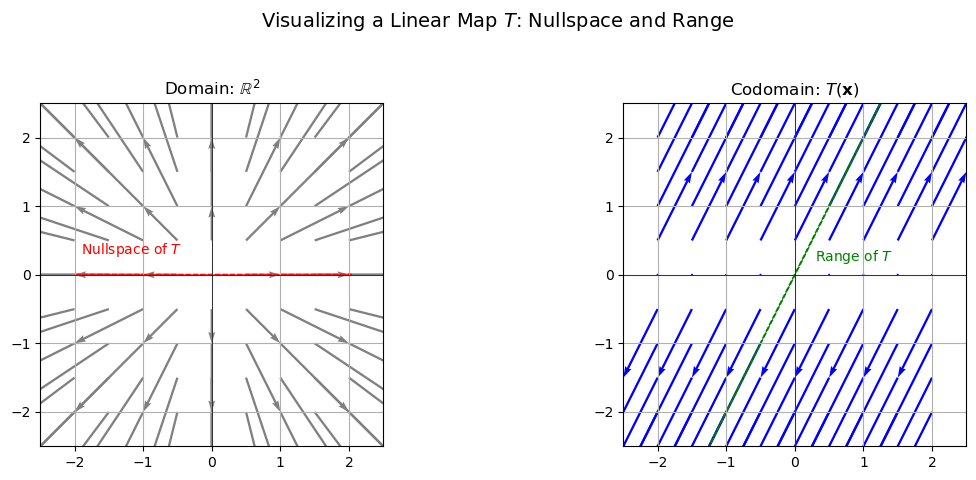
Left Plot: Domain — \(\mathbb{R}^2\)
Grey Arrows:
These arrows represent a grid of input vectors \(\mathbf{x} \in \mathbb{R}^2\). Each arrow is drawn from its base point \((x, y)\) and points in the direction of the vector \(\mathbf{x}\) itself (i.e., the displacement from the origin to \((x, y)\)). This gives a sense of the “structure” of the domain space before applying the linear map \(T\). It’s a regular grid of vectors, all pointing away from the origin, forming a kind of “reference frame” for visualizing the transformation.Red Dashed Arrow: This arrow indicates the nullspace direction of the linear map \(T\). Any vector along this direction gets mapped to zero by \(T\). In this case, it’s the x-axis, which is collapsed to zero in the codomain.
Right Plot: Codomain — \(T(\mathbf{x}) \in \mathbb{R}^2\)
Blue Arrows:
These are the images of the grey vectors after the transformation. For each vector \(\mathbf{x}\) in the domain, we compute \(T(\mathbf{x}) = \mathbf{A}\mathbf{x}\), and draw the resulting vector starting from the same base point \((x, y)\). So for any input vector \(\mathbf{x} = \begin{bmatrix} x \\ y \end{bmatrix}\), we have:
That means the image of every \(\mathbf{x}\) under \(T\) lies on the line:
Theorem (Nullspace of a Linear Map)
The Nullspace \(\operatorname{null}(T)\) is a subspace of \(V\).
Proof. For any linear map \(T: V \to W\):
Define
We need to show that \(\operatorname{null}(T)\) satisfies the three subspace conditions:
(i) Contains the zero vector:
Since \(T\) is linear,
Hence, \(\mathbf{0} \in \operatorname{null}(T)\).
(ii) Closed under vector addition:
Let \(\mathbf{x}, \mathbf{y} \in \operatorname{null}(T)\). Then, by the definition of the nullspace,
Since \(T\) is linear,
Thus, \(\mathbf{x} + \mathbf{y} \in \operatorname{null}(T)\).
(iii) Closed under scalar multiplication:
Let \(\mathbf{x} \in \operatorname{null}(T)\) and let \(\alpha \in \mathbb{R}\). Then,
By linearity,
Hence, \(\alpha \mathbf{x} \in \operatorname{null}(T)\).
Since all three conditions are met, \(\operatorname{null}(T)\) is a subspace of \(V\).
Theorem (Range of a Linear Map)
The Range \(\operatorname{range}(T)\) is a subspace of \(W\).
Proof. For any linear map \(T: V \to W\): Define
Again, we check the subspace properties:
(i) Contains the zero vector:
Since \(T\) is linear,
implying that \(\mathbf{0} \in \operatorname{range}(T)\) (choose \(\mathbf{x} = \mathbf{0}\)).
(ii) Closed under vector addition:
Let \(\mathbf{y}_1, \mathbf{y}_2 \in \operatorname{range}(T)\). Then there exist \(\mathbf{x}_1, \mathbf{x}_2 \in V\) such that
By linearity,
Therefore, \(\mathbf{y}_1 + \mathbf{y}_2 \in \operatorname{range}(T)\).
(iii) Closed under scalar multiplication:
Let \(\mathbf{y} \in \operatorname{range}(T)\) and let \(\alpha \in \mathbb{R}\). Then there exists \(\mathbf{x} \in V\) such that
By linearity,
Hence, \(\alpha \mathbf{y} \in \operatorname{range}(T)\).
Since \(\operatorname{range}(T)\) contains the zero vector and is closed under both vector addition and scalar multiplication, it is a subspace of \(W\).
The rank of a linear map \(T\) is the dimension of its range, and the nullity of \(T\) is the dimension of its nullspace.
Theorem (Rank-Nullity Theorem)
For a linear map \(T: V \to W\), the rank of \( T \) (i.e. the number of linearly independent columns in the matrix representation of \( T \)) is exactly the dimension of its range (or column space) and the nullity of \( T \) is the dimension of its nullspace (kernel).
The rank-nullity theorem is a fundamental result in linear algebra that relates the dimensions of the nullspace and range of a linear map to the dimension of its domain. It is particularly useful in understanding the structure of linear transformations and their effects on vector spaces. We omit the proof for now, until we have introduced the singular value decomposition (SVD) of a matrix that will make the proof much easier.
Affine Subspaces#
A subspace \( S \) of a vector space \( V \) is, by definition, a set that contains the zero vector and is closed under vector addition and scalar multiplication. In many practical settings—such as when applying linear maps it is useful to consider sets of points that are “shifted” from a true subspace. These are called affine subspaces.
An affine subspace of \( V \) is a set that can be written in the form
where \( U \subseteq V \) is a subspace and \( \mathbf{v}_0 \in V \) is a fixed vector. Although an affine subspace is “flat” (it has the same geometric structure as \( U \)), it is not a subspace in the strict sense because it does not necessarily contain the zero vector—unless \( \mathbf{v}_0 = \mathbf{0} \).
Key Properties#
Translation of a Subspace:
Every affine subspace is a translation of a linear subspace \( U \). The vector \( \mathbf{v}_0 \) “shifts” \( U \) so that the resulting affine subspace need not pass through the origin.Failure of Closure Under Scalar Multiplication:
While \( U \) is closed under scalar multiplication, \( \mathbf{v}_0 + U \) is not. For example, if \( \mathbf{x} \in \mathbf{v}_0 + U \), then \( \alpha \mathbf{x} \) is generally not in \( \mathbf{v}_0 + U \) unless \( \mathbf{v}_0 = \mathbf{0} \).Affine Combinations:
Even though an affine subspace is not a vector space, it is closed under affine combinations. That is, if \(\mathbf{x}_1, \dots, \mathbf{x}_k\) belong to the affine subspace \( \mathbf{v}_0 + U \) and \(\lambda_1,\dots,\lambda_k\) are real numbers with \(\sum_{i=1}^k \lambda_i = 1\), then\[\sum_{i=1}^k \lambda_i \mathbf{x}_i \in \mathbf{v}_0 + U.\]Dimension: The dimension of an affine subspace is the same as that of the subspace \( U \). If \( U \) is \( k \)-dimensional, then the affine subspace \( \mathbf{v}_0 + U \) is also \( k \)-dimensional.
Intersection with a Subspace: The intersection of an affine subspace with a linear subspace is either empty or an affine subspace itself. This is because the intersection can be expressed as a translation of the original subspace.
Examples#
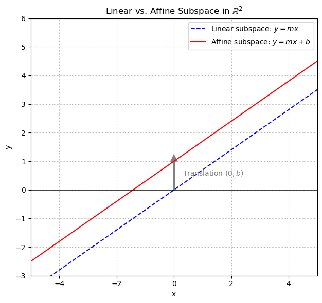
Line in \(\mathbb{R}^2\):
A line through the origin is a subspace. However, a line that does not pass through the origin is an affine subspace. For instance, the set\[ \{(x,y) \in \mathbb{R}^2 : y = mx + b\} \]with \(b \neq 0\) defines an affine subspace of \(\mathbb{R}^2\) since it is a translation of the line \(y = mx\) by the vector \((0,b)\). It can equivalently be expressed as
\[ (0, b) + \{ (x, mx) \mid x \in \mathbb{R} \}. \]
Show code cell source
import numpy as np
import matplotlib.pyplot as plt

# Parameters of the lines
m = 0.7   # slope
b = 1.0   # vertical shift for the affine subspace

# x range for plotting
x_vals = np.linspace(-5, 5, 400)

# Compute y values for linear and affine subspaces
y_linear = m * x_vals
y_affine = m * x_vals + b

# Plotting
plt.figure(figsize=(8, 6))
plt.plot(x_vals, y_linear, label=r"Linear subspace: $y = mx$", color='blue', linestyle='--')
plt.plot(x_vals, y_affine, label=r"Affine subspace: $y = mx + b$", color='red')

# Mark the translation vector (0, b)
plt.arrow(0, 0, 0, b, head_width=0.2, head_length=0.2, fc='gray', ec='gray', linestyle='-', linewidth=2)
plt.text(0.3, b / 2, r"Translation $(0,b)$", color='gray')

# Axis configuration
plt.axhline(0, color='black', linewidth=0.5)
plt.axvline(0, color='black', linewidth=0.5)
plt.grid(True, linestyle=':')
plt.gca().set_aspect('equal', adjustable='box')
plt.xlim(-5, 5)
plt.ylim(-3, 6)

# Labels and legend
plt.xlabel("x")
plt.ylabel("y")
plt.title(r"Linear vs. Affine Subspace in $\mathbb{R}^2$")
plt.legend()
plt.tight_layout()
plt.show()
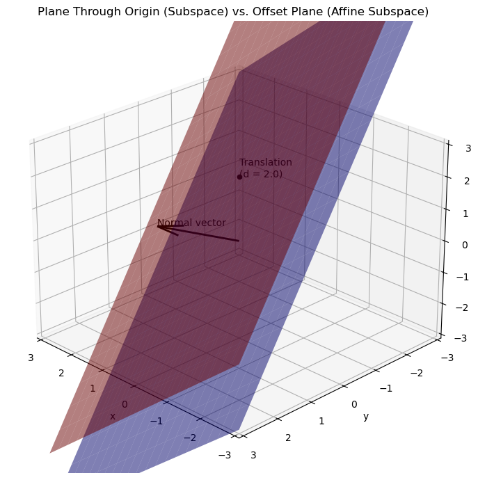
Plane in \(\mathbb{R}^3\):
A plane that passes through the origin is a subspace of \(\mathbb{R}^3\). Conversely, a plane defined as\[ \{\mathbf{x} \in \mathbb{R}^3 : \mathbf{n}^\top \mathbf{x} = d\}, \quad d \neq 0, \]is an affine subspace because it does not contain the zero vector unless \(d = 0\).
Show code cell source
import numpy as np
import matplotlib.pyplot as plt
from mpl_toolkits.mplot3d import Axes3D

# Define normal vector and offset
n = np.array([1, 2, 1])  # plane normal
d = 2.0  # offset for affine subspace (must be != 0)

# Create a grid of x, y values
x_vals = np.linspace(-3, 3, 20)
y_vals = np.linspace(-3, 3, 20)
X, Y = np.meshgrid(x_vals, y_vals)

# Plane through origin (linear subspace): n^T x = 0 -> solve for z
Z_linear = (-n[0] * X - n[1] * Y) / n[2]

# Affine subspace: n^T x = d -> solve for z
Z_affine = (-n[0] * X - n[1] * Y + d) / n[2]

# Set up 3D plot
fig = plt.figure(figsize=(10, 7))
ax = fig.add_subplot(111, projection='3d')

# Plot the plane through origin
ax.plot_surface(X, Y, Z_linear, color='blue', alpha=0.5, label='Linear subspace')

# Plot the affine plane
ax.plot_surface(X, Y, Z_affine, color='red', alpha=0.5)

# Add the normal vector
normal_origin = np.array([[0], [0], [0]])
normal_tip = n / np.linalg.norm(n) * d
ax.quiver(*normal_origin.flatten(), *normal_tip, color='black', linewidth=2)
ax.text(*normal_tip, "Normal vector", color='black')

# Plot a reference point on affine plane
x0 = np.array([0, 0, d / n[2]])
ax.scatter(*x0, color='black')
ax.text(*x0, f"Translation\n(d = {d})", color='black')

# Labels and formatting
ax.set_xlabel('x')
ax.set_ylabel('y')
ax.set_zlabel('z')
ax.set_title("Plane Through Origin (Subspace) vs. Offset Plane (Affine Subspace)")
ax.view_init(elev=25, azim=135)
ax.set_xlim(-3, 3)
ax.set_ylim(-3, 3)
ax.set_zlim(-3, 3)

plt.tight_layout()
plt.show()
Formal Observation#
If \(S\) is an affine subspace of \(V\) represented as \(S = \mathbf{v}_0 + U\), then for any \(\mathbf{x}, \mathbf{y} \in S\), the difference \(\mathbf{x} - \mathbf{y}\) lies in the subspace \(U\). This property allows us to “recover” the linear structure from an affine one.
In summary, affine subspaces are “shifted” linear subspaces: they maintain the geometric flatness (lines, planes, etc.) but may not include the origin.
Hyperplanes and Linear Classification#
In linear classifiers the decision boundary is a linear function separating the classes. For binary classification, such as distinguishing benign from malignant biopsies, the decision boundary separates the space into two halfspaces.
A Hyperplane in Euclidean Space#
In an \(n\)-dimensional Euclidean space \(\mathbb{R}^n\), a hyperplane is a flat, \((n-1)\)-dimensional subset that divides the space into two distinct halfspaces.
Formally, a hyperplane can be expressed as:
where:
\(\mathbf{w} \in \mathbb{R}^n\) is a normal vector perpendicular to the hyperplane.
\(b \in \mathbb{R}\) is a scalar offset determining the hyperplane’s position relative to the origin.
A halfspace in \(\mathbb{R}^n\) is defined by:
Where:
\(\mathbf{w}\) is a vector perpendicular to the decision boundary
\(b\) is a scalar offset
Affine Subspace:
A hyperplane is a linear manifold but not a subspace unless it passes exactly through the origin. Generally, this hyperplane does not contain the zero vector, and hence it violates condition (i) of the subspace definition. However, it is an affine subspace of \(\mathbb{R}^n\), as it can be expressed as:
Given \(\mathbf{w} \in \mathbb{R}^n\) (with \(\mathbf{w} \neq \mathbf{0}\)) and a scalar \(b\), a particular solution \(\mathbf{x}_0\) of the equation
must satisfy \(\mathbf{w}^\top \mathbf{x}_0 = -b\). A standard way to obtain such an \(\mathbf{x}_0\) is to set:
Notice that \(\|\mathbf{w}\|^2 = \mathbf{w}^\top \mathbf{w}\) is a scalar (and not \(\mathbf{w}^\top\) by itself), which makes the fraction well defined. Indeed,
as required.
Every \(\mathbf{x}\) satisfying the hyperplane equation can be written as
where \(\mathbf{u}\) is any vector in the subspace
In other words, \(U\) is the \((n-1)\)-dimensional subspace orthogonal to \(\mathbf{w}\). This shows that the hyperplane is an affine subspace—that is, it is a translation of the linear subspace \(U\) by the vector \(\mathbf{x}_0\).
The hyperplane can be written as:
This expression decomposes any point on the hyperplane into a particular solution plus a component that lies in the \((n-1)\)-dimensional subspace \(U\).
Subspaces of the Space of Functions#
Beyond vector spaces of finite-dimensional vectors like \(\mathbb{R}^n\), we can also consider vector spaces whose elements are functions. In particular, let us define the set:
This set contains all real-valued functions on \(\mathbb{R}^d\), and it forms an infinite-dimensional vector space:
The zero function \(f(\mathbf{x}) = 0\) is in \(\mathcal{F}\)
If \(f, g \in \mathcal{F}\), then \(f + g \in \mathcal{F}\)
If \(f \in \mathcal{F}\) and \(\alpha \in \mathbb{R}\), then \(\alpha f \in \mathcal{F}\)
While \(\mathcal{F}\) is too large to work with directly in most learning problems, we can identify useful subspaces of \(\mathcal{F}\) that play an important role in machine learning.
Subspace 1: Functions Spanned by Basis Functions#
Let \(\phi_1, \dots, \phi_k\) be fixed basis functions, such as polynomials, splines, or radial basis functions (RBFs), each mapping \(\mathbb{R}^d \to \mathbb{R}\). Then the set:
forms a finite-dimensional subspace of \(\mathcal{F}\). This subspace is central to many machine learning models, such as polynomial regression, kernel methods, and additive models.
It contains the zero function (when all \(\theta_i = 0\))
It is closed under addition and scalar multiplication
It provides a way to parametrize functions via their coefficients \(\boldsymbol{\theta} \in \mathbb{R}^k\)
Subspace 2: Affine Functions Learned by Linear Regression#
Linear regression can also be interpreted as learning a function in a subspace of \(\mathcal{F}\). The learned function has the form:
This defines an affine function, but if we include a constant basis function (i.e., append a 1 to \(\mathbf{x}\)), this becomes a linear function in an extended space:
The set of all such functions is a \((d+1)\)-dimensional subspace of \(\mathcal{F}\), and corresponds exactly to the set of functions learnable by ordinary least squares linear regression (with bias).
Why Restrict to Subspaces?#
Working directly in \(\mathcal{F}\) is intractable: we cannot learn arbitrary functions from finite data. Restricting to a subspace of \(\mathcal{F}\) gives us:
Finite representations (via weights or coefficients)
Efficient computation (linear algebra instead of function space calculus)
Better generalization (we avoid overfitting by limiting complexity)
This is why almost all models in machine learning — from linear models to neural networks and kernel machines — effectively learn within a structured, finite-dimensional subspace of the function space \(\mathcal{F}\).
By understanding these subspaces, we gain insight into what a model can express, how it generalizes, and how it relates to geometric structures like subspaces of vector spaces.
Summary#
A subspace of a vector space \(V\) is a subset that is closed under addition and scalar multiplication, and contains the zero vector.
The nullspace and range of a linear map are subspaces of the domain and codomain, respectively.
The rank-nullity theorem relates the dimensions of the nullspace and range to the dimension of the domain.
An affine subspace is a translation of a linear subspace and does not necessarily contain the zero vector.
Affine combinations are closed in affine subspaces, but not in linear subspaces.
Subspaces of function spaces are important in machine learning, allowing us to work with finite-dimensional representations of functions.