Extrema

Optimization is about finding extrema, which depending on the application could be minima or maxima. When defining extrema, it is necessary to consider the set of inputs over which we’re optimizing.

Unconstrained vs. Constrained Optimization

This set \(\mathcal{X} \subseteq \mathbb{R}^d\) is called the feasible set. If \(\mathcal{X}\) is the entire domain of the function being optimized (as it often will be for our purposes), we say that the problem is unconstrained. Otherwise the problem is constrained and may be much harder to solve, depending on the nature of the feasible set.

In the following example we observe the difference in optimization of the function \(f(x,y)=(x-1)^2+2(y-2)^2\) over all of \(\mathbb{R}^2\) from constrained optimization over a subset \(\mathcal{X}=\{(x,y)\|x^2+y^2\leq 4\}\), with the constrained problem leading the minimizer to lie on the boundary of the feasible region.

Show code cell source Hide code cell source

import numpy as np
import matplotlib.pyplot as plt
from matplotlib.patches import Circle

# Define the objective function f(x, y) = (x-1)^2 + 2*(y-2)^2
def f(x, y):
    return (x - 1)**2 + 2*(y - 2)**2

# Unconstrained minimum at (1,2)
unconstrained_min = np.array([1.0, 2.0])

# Feasible set: disk of radius 2 centered at the origin
radius = 2.0

# Constrained minimum: projection onto the disk if outside
norm_uc = np.linalg.norm(unconstrained_min)
if norm_uc <= radius:
    constrained_min = unconstrained_min.copy()
else:
    constrained_min = unconstrained_min / norm_uc * radius

# Create a grid for contour plotting
x_vals = np.linspace(-3, 3, 400)
y_vals = np.linspace(-3, 3, 400)
X, Y = np.meshgrid(x_vals, y_vals)
Z = f(X, Y)

# Plot contours of the objective
plt.figure(figsize=(8, 8))
contours = plt.contour(X, Y, Z, levels=30, cmap='viridis')
plt.clabel(contours, inline=True, fontsize=8)

# Draw the feasible set
ax = plt.gca()
disk = Circle((0, 0), radius, color='orange', alpha=0.3, label='Feasible set\n$x^2+y^2 \\leq 4$')
ax.add_patch(disk)

# Plot the minima
plt.scatter(*unconstrained_min, color='red', s=100, label='Unconstrained minimum\n$(1,2)$')
plt.scatter(*constrained_min, color='blue', s=100, label='Constrained minimum\non disk')

# Annotate points
plt.text(unconstrained_min[0]+0.1, unconstrained_min[1]+0.1, 'Unconstrained', color='red')
plt.text(constrained_min[0]+0.1, constrained_min[1]+0.1, 'Constrained', color='blue')

# Final formatting
plt.title('Unconstrained vs. Constrained Optimization\nand the Feasible Set')
plt.xlabel('$x$')
plt.ylabel('$y$')
plt.legend(loc='lower right')
plt.grid(True, linestyle=':')
plt.xlim(-2.5, 2.5)
plt.ylim(-2.5, 2.5)
plt.gca().set_aspect('equal', adjustable='box')
plt.tight_layout()
plt.show()

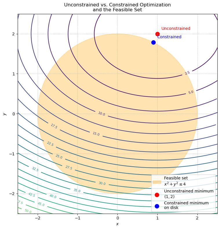
• The level curves (contours) of the cost function \(f(x,y)=(x-1)^2+2(y-2)^2\).

• The unconstrained minimum (red) at \((1,2)\), which lies outside the feasible disk.

• The feasible set (orange disk) defined by \(x^2+y^2 \le 2^2\).

• The constrained minimum (blue) as the projection of the unconstrained solution onto the disk boundary.

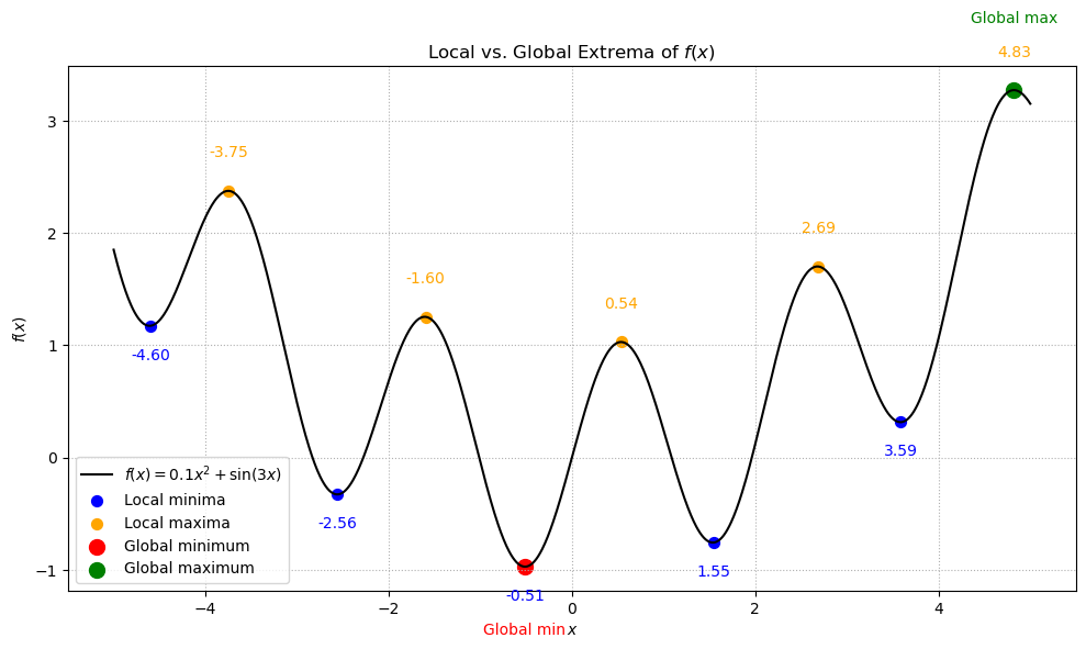
Local vs. Global Extrema

Suppose \(f : \mathbb{R}^d \to \mathbb{R}\). A point \(\mathbf{x}\) is said to be a local minimum (resp. local maximum) of \(f\) in \(\mathcal{X}\) if \(f(\mathbf{x}) \leq f(\mathbf{y})\) (resp. \(f(\mathbf{x}) \geq f(\mathbf{y})\)) for all \(\mathbf{y}\) in some neighborhood \(N \subseteq \mathcal{X}\) about \(\mathbf{x}\).

Furthermore, if \(f(\mathbf{x}) \leq f(\mathbf{y})\) for all \(\mathbf{y} \in \mathcal{X}\), then \(\mathbf{x}\) is a global minimum of \(f\) in \(\mathcal{X}\) (similarly for global maximum). If the phrase “in \(\mathcal{X}\)” is unclear from context, assume we are optimizing over the whole domain of the function.

The qualifier strict (as in e.g. a strict local minimum) means that the inequality sign in the definition is actually a \(>\) or \(<\), with equality not allowed. This indicates that the extremum is unique within some neighborhood.

Here’s an example visualization of the one‑dimensional function \(f(x)=0.1x^2+\sin(3x)\), which has several “valleys” and “peaks” that correspond to local minima and maxima:

Show code cell source Hide code cell source

import numpy as np
import matplotlib.pyplot as plt

# 1D function with multiple extrema
def f(x):
    # Quadratic tilt + oscillation
    return 0.1 * x**2 + np.sin(3*x)

# Sample the function
x = np.linspace(-5, 5, 1000)
y = f(x)

# Approximate derivatives
dy = np.gradient(y, x)
d2y = np.gradient(dy, x)

# Detect local minima: derivative sign change from - to + and positive curvature
local_min_idx = np.where((dy[:-1] < 0) & (dy[1:] > 0) & (d2y[:-1] > 0))[0] + 1
# Detect local maxima: derivative sign change from + to - and negative curvature
local_max_idx = np.where((dy[:-1] > 0) & (dy[1:] < 0) & (d2y[:-1] < 0))[0] + 1

# Detect global extrema
global_min_idx = np.argmin(y)
global_max_idx = np.argmax(y)

# Plot the function
plt.figure(figsize=(10, 6))
plt.plot(x, y, 'k-', linewidth=1.5, label=r'$f(x)=0.1x^2+\sin(3x)$')

# Mark local minima and maxima
plt.scatter(x[local_min_idx], y[local_min_idx], c='blue', s=50, label='Local minima')
plt.scatter(x[local_max_idx], y[local_max_idx], c='orange', s=50, label='Local maxima')

# Mark global minimum and maximum
plt.scatter(x[global_min_idx], y[global_min_idx], c='red',   s=100, label='Global minimum')
plt.scatter(x[global_max_idx], y[global_max_idx], c='green', s=100, label='Global maximum')

# Annotate points with their x‐coordinates
for idx in local_min_idx:
    plt.text(x[idx], y[idx] - 0.3, f"{x[idx]:.2f}", color='blue', ha='center')
for idx in local_max_idx:
    plt.text(x[idx], y[idx] + 0.3, f"{x[idx]:.2f}", color='orange', ha='center')
plt.text(x[global_min_idx], y[global_min_idx] - 0.6, 'Global min', color='red', ha='center')
plt.text(x[global_max_idx], y[global_max_idx] + 0.6, 'Global max', color='green', ha='center')

# Final formatting
plt.title('Local vs. Global Extrema of $f(x)$')
plt.xlabel('$x$')
plt.ylabel('$f(x)$')
plt.legend()
plt.grid(True, linestyle=':')
plt.tight_layout()
plt.show()