Multivariate Calculus in Machine Learning#
Before we dive into the formal definitions of extrema and unconstrained optimization, let’s see how this all ties back to machine learning.
In machine learning we often have a loss function \(\ell(y,\,\hat{y})\) that measures the discrepancy between a true label \(y\) and a predicted label \(\hat{y}\) that is the output of a parameteriyed function \(\hat{y}=f(\mathbf{x};\,\boldsymbol{\theta})\), where \(\mathbf{x}\) is the input feature vector. The loss function is typically a function of both the true label \(y\) and the predicted label \(\hat{y}\), and it can take different forms depending on the type of problem we are solving.
For example, in regression, we might use the squared error loss
and in classification, we might use the logistic loss
In both cases, \(\ell\) is a function of the predicted label \(\hat{y}\), which is itself a function of the model parameters \(\boldsymbol{\theta}\) and the input data \(\mathbf{x}\). Thus, we can write the loss as a function of the model parameters:
or
In this context, \(\boldsymbol{\theta}\) is a vector of parameters (weights) that we want to optimize. The goal of supervised learning is to find the optimal parameters \(\boldsymbol{\theta}^*\) that minimize the expected loss over the data distribution. This is often referred to as risk minimization.
Our ultimate goal is to minimize the true risk
which depends on the unknown data‐generating distribution \(P\). Since \(P\) is not accessible, we instead minimize the empirical risk based on a finite sample of data points \(\{(\mathbf{x}_i,y_i)\}_{i=1}^n\) drawn from \(P\):
This is the essence of empirical risk minimization (ERM), a fundamental principle in machine learning. The idea is to find the parameters \(\boldsymbol{\theta}^*\) that minimize the empirical risk, which serves as an approximation of the true risk. \(R_{\mathrm{emp}}(\boldsymbol{\theta})\) is a function \(\mathbb{R}^d\to\mathbb{R}\) of the \(d\) parameters, and finding the best model amounts to finding the global minimum of \(R_{\mathrm{emp}}(\boldsymbol{\theta})\) (or a good local minimum, in non‑convex settings).
Minimization of the empirical risk is a common approach in machine learning, and it is often done using optimization algorithms such as gradient descent. The idea is to iteratively update the parameters \(\boldsymbol{\theta}\) in the direction of the negative gradient of the empirical risk until convergence.
To illustrate this, we show gradient descent applied to the empirical risk \(R_{\mathrm{emp}}(\mathbf{w})\) and the corresponding unkown true risk \(R(\mathbf{w})\) for a simple linear regression problem for each step of the gradient descent algorithm:
Show code cell source
import numpy as np
import matplotlib.pyplot as plt

# bias


# linear component
slope = 2

# cyclical component
frequency = 3
amplitude = 0.1
phase_shift = 1

# iid Gaussian Noise
noise_std = 1.5

# Generate synthetic data for linear regression (1D feature)
np.random.seed(0)
n = 20
left_bound = -1 # lower bound of uniform distribution on X
right_bound = 1 # upper bound of uniform distribution on X
X = np.random.uniform(left_bound, right_bound, n)
y = slope * X # noise-free y
y += np.random.randn(n) * noise_std  # add iid noise
# + amplitude*np.sin(phase_shift + frequency*X)

# Define the empirical risk (mean squared error) and its derivative
def R_emp(w):
    return np.mean((y - w * X)**2)

def grad_R_emp(w):
    return np.mean(-2 * X * (y - w * X))

# Grid of w values
w_vals = np.linspace(-3, 3, 400)
R_emp_vals = np.array([R_emp(w) for w in w_vals])

# True risk (expected risk) for this synthetic model
# E_x[(slope*x - w x)^2] + Var(noise) = (w - slope)^2 * E[x^2] + sigma^2
sigma2 = noise_std**2
E_x2 = (left_bound - right_bound)**2 / 12   # variance of uniform distribution
R_true_vals = (w_vals - slope)**2 * E_x2 + sigma2

# Gradient descent on empirical risk
lr = 0.1
convergence_criterion = 1e-6
num_steps = 500
w_path = [-3.0]
for _ in range(num_steps):
    w_curr = w_path[-1]
    gradient =  grad_R_emp(w_curr)
    w_next = w_curr - lr * gradient
    w_path.append(w_next)
    if np.linalg.norm(gradient)<convergence_criterion:
        break
w_path = np.array(w_path)
R_path = np.array([R_emp(w) for w in w_path])

# Plot empirical and true risk, plus descent path
plt.figure(figsize=(8, 6))
plt.plot(w_vals, R_emp_vals, label="Empirical Risk $R_{emp}(w)$")
plt.plot(w_vals, R_true_vals, '--', label="True Risk $R(w)$", color='gray')
plt.plot(w_path, R_path, 'o-', color='C1', label="Gradient Descent on $R_{emp}$")
for i in range(len(w_path)-1):
    plt.arrow(w_path[i], R_path[i],
              w_path[i+1] - w_path[i], R_path[i+1] - R_path[i],
              head_width=0.1, head_length=0.05, fc='C1', ec='C1')

plt.scatter([w_path[0]], [R_path[0]], color='black', zorder=5, label="Start")
plt.scatter([w_path[-1]], [R_path[-1]], color='red', zorder=5, label="Converged")

plt.title("Empirical vs. True Risk and Gradient Descent Trajectory")
plt.xlabel("Parameter $w$")
plt.ylabel("Risk")
plt.legend()
plt.grid(True, linestyle=':')
plt.tight_layout()
plt.show()
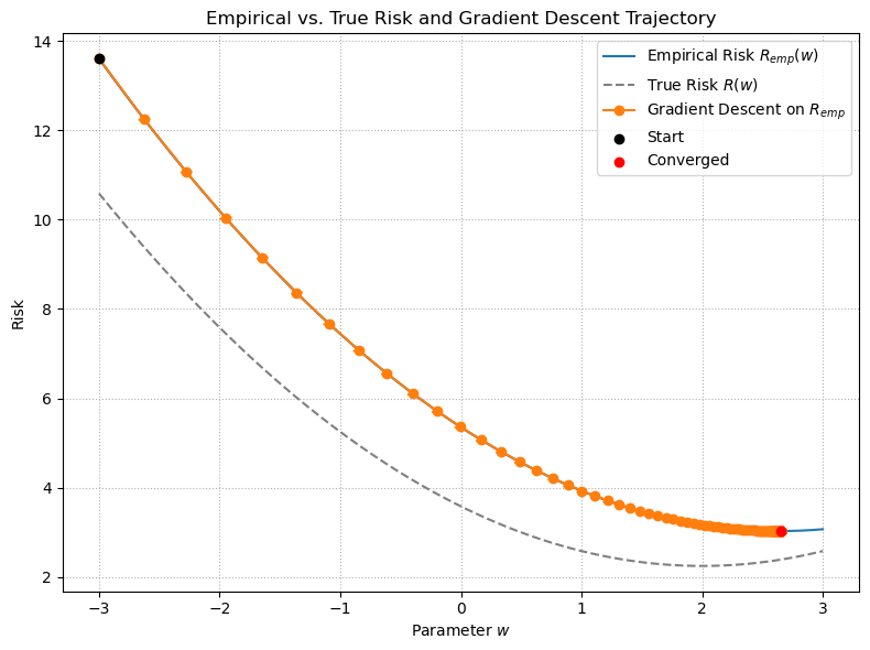
The plot above shows how \(R_{\mathrm{emp}}(w)\) (solid orange) approximates the unkown true risk \(R(w)\) (dashed gray) for a simple linear model with quadratic loss. Gradient descent on \(R_{\mathrm{emp}}\) converges to a minimizer of the empirical risk (red “Converged” point).
Key implications:
Approximation error: Because we only minimize \(R_{\mathrm{emp}}\), our solution may not exactly minimize the true risk.
Overfitting vs. generalization: A model that perfectly minimizes \(R_{\mathrm{emp}}\) (especially with limited data) can overfit, achieving low training error but higher true risk on new data.
Statistical guarantees: Under standard assumptions (e.g. i.i.d.\ sampling, sufficient data), \(R_{\mathrm{emp}}\) converges uniformly to \(R\) as \(n\to\infty\), and minimizers of the empirical risk converge to minimizers of the true risk.
Observe that maximizing a function \(g\) (such as a log-likelihood function of a probabilistic model) is equivalent to minimizing \(-g\),so optimization problems are typically phrased in terms of minimization without loss of generality. This convention (which we follow here) eliminates the need to discuss minimization and maximization separately.
Thus, in machine learning, the entire machinery of multivariate calculus, gradients, Jacobians, Hessians, and descent algorithms is in service of empirical risk minimization: we view training as an optimization problem over a high‑dimensional parameter space, seeking the parameter vector \(\boldsymbol{\theta}^*\) that minimizes our cost function (also called an objective function). With this motivation in mind, we now recall the basic definitions of extrema, local versus global minima, gradients and Hessians.