The Hessian

In one variable, the second derivative of a function is a number that tells us about the curvature of the function. But in many variables, each partial derivative can change in many directions—so we need a matrix of second derivatives:

The Hessian matrix of a scalar-valued function \( f : \mathbb{R}^d \to \mathbb{R} \) is a square matrix of second-order partial derivatives:

\[\begin{split}\nabla^2 f(\mathbf{x}) = \begin{bmatrix} \frac{\partial^2 f}{\partial x_1^2} & \dots & \frac{\partial^2 f}{\partial x_1 \partial x_d} \\ \vdots & \ddots & \vdots \\ \frac{\partial^2 f}{\partial x_d \partial x_1} & \dots & \frac{\partial^2 f}{\partial x_d^2} \end{bmatrix}, \quad\text{i.e.,}\quad [\nabla^2 f]_{ij} = \frac{\partial^2 f}{\partial x_i \partial x_j} \end{split}\]

Theorem (Clairaut Schwarz)

Let \(f: \mathbb{R}^d \to \mathbb{R}\) be a function such that both mixed partial derivatives \(\frac{\partial^2 f}{\partial x_i \partial x_j}\) and \(\frac{\partial^2 f}{\partial x_j \partial x_i}\) exist and are continuous on an open set containing a point \(\mathbf{x}_0\)

Then:

\[ \boxed{ \frac{\partial^2 f}{\partial x_i \partial x_j}(\mathbf{x}_0) = \frac{\partial^2 f}{\partial x_j \partial x_i}(\mathbf{x}_0) } \]

That is, the order of differentiation can be interchanged.

Clairut’s Theorem implies that the Hessian matrix is symmetric. We provide a proof sketch in the appendix.

Curvature in One Dimension

Recall the second derivative in one dimension:

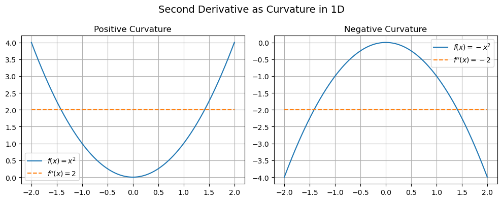
• \(f(x) = x^2\): curve is “smiling” ⇒ second derivative is positive ⇒ function is curving upward.

• \(f(x) = -x^2\): curve is “frowning” ⇒ second derivative is negative ⇒ function is curving downward.

• Point: second derivative tells us how the function curves.

Show code cell source Hide code cell source

import numpy as np
import matplotlib.pyplot as plt

x = np.linspace(-2, 2, 400)
f1 = x**2
f2 = -x**2
f1_dd = np.full_like(x, 2)   # Second derivative of x^2
f2_dd = np.full_like(x, -2)  # Second derivative of -x^2

fig, axes = plt.subplots(1, 2, figsize=(10, 4))

# Plot for f(x) = x^2
axes[0].plot(x, f1, label='$f(x) = x^2$')
axes[0].plot(x, f1_dd, '--', label='$f\'\'(x) = 2$')
axes[0].set_title('Positive Curvature')
axes[0].legend()
axes[0].grid(True)

# Plot for f(x) = -x^2
axes[1].plot(x, f2, label='$f(x) = -x^2$')
axes[1].plot(x, f2_dd, '--', label='$f\'\'(x) = -2$')
axes[1].set_title('Negative Curvature')
axes[1].legend()
axes[1].grid(True)

plt.suptitle("Second Derivative as Curvature in 1D", fontsize=14)
plt.tight_layout()
plt.show()

The Hessian generalizes this intuition to multiple Dimensions.

Curvature in Two Dimensions

Now, let’s look at a simple 2D surface like:

• \(f(x, y) = x^2 + y^2\): bowl shape

• \(f(x, y) = x^2 - y^2\): saddle shape

Show code cell source Hide code cell source

from mpl_toolkits.mplot3d import Axes3D
from matplotlib import cm

x = np.linspace(-2, 2, 100)
y = np.linspace(-2, 2, 100)
X, Y = np.meshgrid(x, y)

# Bowl: f(x, y) = x^2 + y^2
Z_bowl = X**2 + Y**2

# Saddle: f(x, y) = x^2 - y^2
Z_saddle = X**2 - Y**2

fig = plt.figure(figsize=(12, 5))

# Bowl surface
ax1 = fig.add_subplot(1, 2, 1, projection='3d')
ax1.plot_surface(X, Y, Z_bowl, cmap=cm.viridis, alpha=0.9)
ax1.set_title("Bowl: $f(x, y) = x^2 + y^2$")
ax1.set_xlabel("x")
ax1.set_ylabel("y")
ax1.set_zlabel("f(x, y)")
# Add annotations for curvature
ax1.text(0, 0, 0, '∂²f/∂x² = 2\n∂²f/∂y² = 2', fontsize=10)

# Saddle surface
ax2 = fig.add_subplot(1, 2, 2, projection='3d')
ax2.plot_surface(X, Y, Z_saddle, cmap=cm.coolwarm, alpha=0.9)
ax2.set_title("Saddle: $f(x, y) = x^2 - y^2$")
ax2.set_xlabel("x")
ax2.set_ylabel("y")
ax2.set_zlabel("f(x, y)")
ax2.text(0, 0, 0, '∂²f/∂x² = 2\n∂²f/∂y² = -2', fontsize=10)

plt.suptitle("Curvature in 2D: Bowl vs Saddle", fontsize=14)
plt.tight_layout()
plt.show()

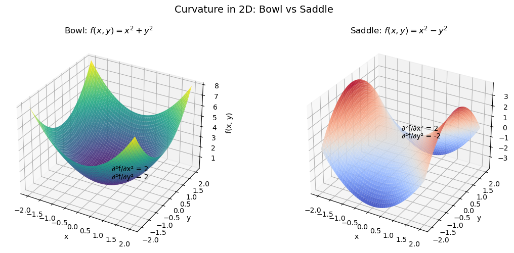
At each point, the function curves more or less in certain directions. The Hessian is a matrix that captures all this curvature information—it tells us how the slope (the gradient) changes in every direction.

---

A Simple Example

\[ f(x, y) = 3x^2 + 2xy + y^2 \]

• \(\frac{\partial f}{\partial x} = 6x + 2y\)

• \(\frac{\partial f}{\partial y} = 2x + 2y\)

• Hessian:

  \[\begin{split} \nabla^2 f = \begin{bmatrix} 6 & 2 \\ 2 & 2 \end{bmatrix} \end{split}\]

Each entry corresponds to a second derivative—either in the x-direction, y-direction, or mixed for the off-diagonals.

Gradient Vector Fields

The Hessian matrix describes how the gradient vector changes as you move through space. Let’s visualize this in a grid with arrows pointing in the direction of the gradient — i.e., where the function increases most steeply.

Show code cell source Hide code cell source

x = np.linspace(-3, 3, 30)
y = np.linspace(-3, 3, 30)
X, Y = np.meshgrid(x, y)

# Gradients
U_bowl = 2 * X
V_bowl = 2 * Y

U_saddle = 2 * X
V_saddle = -2 * Y

fig, axes = plt.subplots(1, 2, figsize=(12, 5))

# Bowl gradient field
axes[0].quiver(X, Y, U_bowl, V_bowl, color='green')
axes[0].set_title('Gradient Field: $f(x, y) = x^2 + y^2$')
axes[0].set_xlabel('x')
axes[0].set_ylabel('y')
axes[0].axis('equal')
axes[0].grid(True)
axes[0].set_ylim([-2.3,2.3])
axes[0].set_xlim([-2.3,2.3])

# Saddle gradient field
axes[1].quiver(X, Y, U_saddle, V_saddle, color='blue')
axes[1].set_title('Gradient Field: $f(x, y) = x^2 - y^2$')
axes[1].set_xlabel('x')
axes[1].set_ylabel('y')
axes[1].axis('equal')
axes[1].grid(True)
axes[1].set_ylim([-2.3,2.3])
axes[1].set_xlim([-2.3,2.3])


plt.suptitle("Gradient Vector Fields Show How ∇f Changes", fontsize=14)
plt.tight_layout()
plt.show()

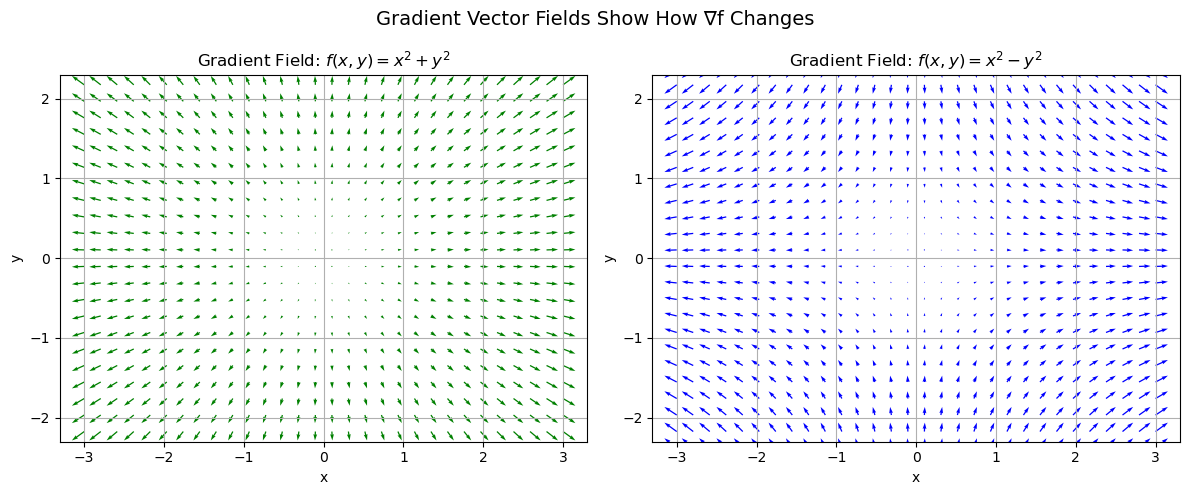
• The gradient vector field shows how gradients vary over space.

• The Hessian is the rate of change of the gradient—it tells you how steep the slope is getting in every direction.

• The direction and length of arrows = the gradient vector at each point.

• The rate of change of those arrows = what the Hessian captures.

---

🔍 How This Works in the Two Examples

🟢 Bowl: \(f(x, y) = x^2 + y^2\)

• Gradient: \(\nabla f(x, y) = [2x,\ 2y]\)

• Hessian:

  \[\begin{split} \nabla^2 f = \begin{bmatrix} 2 & 0 \\ 0 & 2 \end{bmatrix} \end{split}\]

This means:

• In the x-direction, the gradient increases by 2 units per unit of x.

• In the y-direction, the gradient increases by 2 units per unit of y.

• The gradient field shows arrows pointing radially outward—getting longer linearly with distance from the origin.

• This linear increase in slope is exactly what the constant entries (2) in the Hessian mean.

🔵 Saddle: \(f(x, y) = x^2 - y^2\)

• Gradient: \(\nabla f(x, y) = [2x,\ -2y]\)

• Hessian:

  \[\begin{split} \nabla^2 f = \begin{bmatrix} 2 & 0 \\ 0 & -2 \end{bmatrix} \end{split}\]

This means:

• In the x-direction, the gradient increases at the same rate as before: 2 per unit of x.

• In the y-direction, the gradient decreases (negative rate): -2 per unit of y.

• The gradient field shows outward arrows in the x-direction, but inward arrows in the y-direction.

• That flip in sign in the Hessian entry \(\partial^2 f/\partial y^2 = -2\) explains why the gradient pulls you toward the origin in y.

🧩 Optional Extension: The Hessian as Jacobian of the Gradient

We can think of the Hessian as the Jacobian of the gradient — it’s the matrix of all partial derivatives of the components of the gradient vector field.

That is:

\[\begin{split} \nabla f(x, y) = \begin{bmatrix} \frac{\partial f}{\partial x} \\ \frac{\partial f}{\partial y} \end{bmatrix} \quad\Rightarrow\quad \nabla^2 f(x, y) = \text{Jacobian}\left( \nabla f(x, y) \right) \end{split}\]

Gradient Descent and the Hessian: Why Off-Diagonal Terms Matter

🧠 Key Idea

Gradient descent minimizes functions by moving in the direction opposite the gradient.

For quadratic functions:

\[ f(x) = \frac{1}{2} x^\top A x \quad \text{with gradient} \quad \nabla f(x) = A x \]

Here, \(A\) is the Hessian matrix, and it determines the shape of level sets and how gradient descent behaves.

• If \(A\) is diagonal → level sets are axis-aligned ellipses (or circles).

• If \(A\) has off-diagonal elements → ellipses are rotated, and gradient descent struggles (zig-zags).

Show code cell source Hide code cell source

import numpy as np
import matplotlib.pyplot as plt

def gradient_descent(A, x0, lr=0.1, steps=30):
    traj = [x0]
    x = x0
    for _ in range(steps):
        grad = A @ x
        x = x - lr * grad
        traj.append(x)
    return np.array(traj)

def plot_descent(A, title, lr=0.1):
    x = np.linspace(-100, 100, 100)
    y = np.linspace(-100, 100, 100)
    X, Y = np.meshgrid(x, y)
    Z = 0.5 * (A[0,0]*X**2 + 2*A[0,1]*X*Y + A[1,1]*Y**2)

    fig, ax = plt.subplots(figsize=(6, 6))
    ax.contour(X, Y, Z, levels=40, cmap='viridis')

    x0 = np.array([80, 90])
    traj = gradient_descent(A, x0, lr=lr, steps=30)
    ax.plot(traj[:,0], traj[:,1], 'ro--', label='GD Path')

    ax.set_title(title)
    ax.set_xlabel('x')
    ax.set_ylabel('y')
    ax.set_aspect('equal')
    ax.grid(True)
    ax.legend()
    plt.show()

Case 1: Spherical Hessian (Identity Matrix)

A_sphere = np.array([[1, 0], [0, 1]])
plot_descent(A_sphere, "Spherical Hessian: $A = I$")

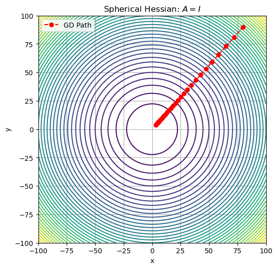
• Level sets are circles.

• Gradient descent takes straight, efficient steps toward the minimum.

Case 2: Anisotropic Hessian (Different Curvatures)

Show code cell source Hide code cell source

A_aniso = np.array([[15, 0], [0, 1]])
plot_descent(A_aniso, "Anisotropic Hessian: $A = \\mathrm{diag}(10, 1)$", lr=0.1)

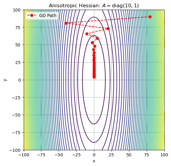
• Level sets are stretched ellipses.

• Gradient descent zig-zags, especially in the steep direction.

---

Case 3: Skewed Hessian (Off-Diagonal Elements)

Show code cell source Hide code cell source

A_skew = np.array([[10, 6], [6, 8]])
plot_descent(A_skew, "Skewed Hessian", lr=0.1)

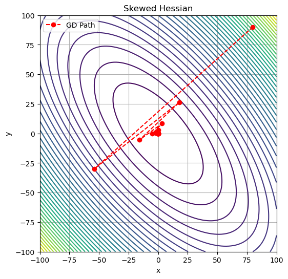
\(A = \begin{bmatrix} 10 & 6 \\ 6 & 8 \end{bmatrix}\)

• Level sets are rotated ellipses.

• Gradient descent strongly zig-zags and converges slowly.

• The skew comes directly from the off-diagonal elements in the Hessian.

Off-diagonal terms in the Hessian rotate the level curves. Since gradient descent moves perpendicular to level curves, it zig-zags when these are skewed. This is one of the motivations for using second-order methods that take the Hessian into account.