Gradients and the Gradient Descent Algorithm#
In this section, we will discuss the concept of gradients and their use in the Steepest Descent optimization algorithm, which is essential in machine learning. Let’s review the basics of derivatives and then move on to partial derivatives and gradients.
Derivatives#
Let \(f:\mathbb{R}\to\mathbb{R}\) be a 1D real-valued function.
The derivative \(f'(x)\) is
if this limit exists.
If \(f'(a)\) exists, we say \(f\) is differentiable at \(a\).
If differentiable for all \(x\) in an interval, we say \(f\) is differentiable on that interval.
\(f'(x)\) is the instantaneous rate of change of \(f\) at \(x\).
\(f'(x)\) is the slope of the tangent line to the graph of \(f\) at \(x\).
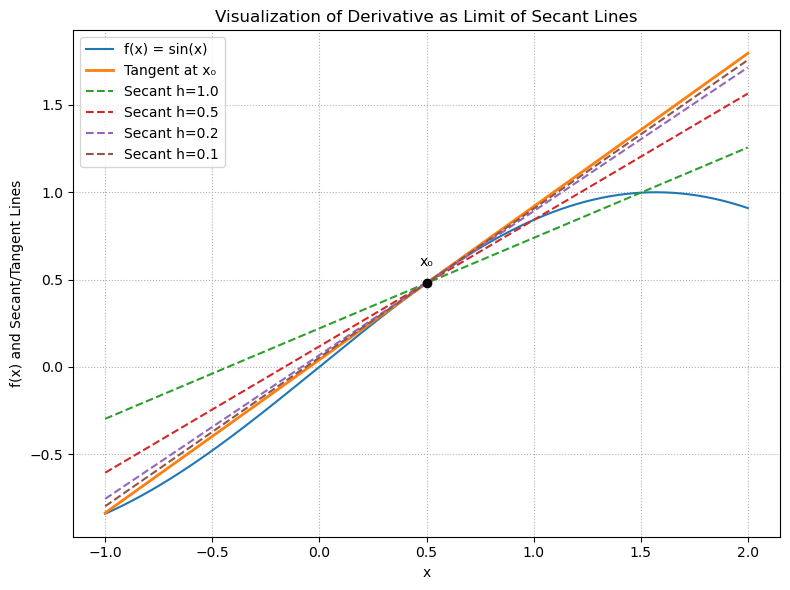
To illustrate the definition of the derivative \(\displaystyle f'(x_0)=\lim_{h\to0}\frac{f(x_0+h)-f(x_0)}{h}\), we can visualize the tangent line of a function at a point \(x_0\) as the limit of secant lines for decreasing \(h\). The secant line between two points \((x_0, f(x_0))\) and \((x_0+h, f(x_0+h))\) has slope
As \(h\) approaches \(0\), the secant line approaches the tangent line at \((x_0, f(x_0))\). The slope of the tangent line is given by the derivative \(f'(x_0)\). To visualize this, we can plot the function \(f(x)=\sin(x)\) and its tangent line at a point \(x_0=0.5\), along with several secant lines for different values of \(h\).
Show code cell source
import numpy as np
import matplotlib.pyplot as plt

# Define the function and its analytical derivative
def f(x):
    return np.sin(x)

def df(x):
    return np.cos(x)

# Choose a point to visualize the derivative
x0 = 0.5
f0 = f(x0)
df0 = df(x0)

# Domain for plotting
x = np.linspace(-1, 2, 400)

# Compute the tangent line at x0
y_tan = f0 + df0 * (x - x0)

# Define a set of h values to illustrate secant lines
h_values = [1.0, 0.5, 0.2, 0.1]

# Set up the plot
plt.figure(figsize=(8, 6))

# Plot the function
plt.plot(x, f(x), label="f(x) = sin(x)")

# Plot the tangent line
plt.plot(x, y_tan, label="Tangent at x₀", linewidth=2)

# Plot secant lines for each h
for h in h_values:
    slope = (f(x0 + h) - f0) / h
    y_sec = f0 + slope * (x - x0)
    plt.plot(x, y_sec, label=f"Secant h={h:.1f}", linestyle='--')

# Mark the point of tangency
plt.scatter([x0], [f0], color='black', zorder=5)
plt.text(x0, f0 + 0.1, "x₀", ha='center')

# Final decorations
plt.title("Visualization of Derivative as Limit of Secant Lines")
plt.xlabel("x")
plt.ylabel("f(x) and Secant/Tangent Lines")
plt.legend()
plt.grid(True, linestyle=':')
plt.tight_layout()
plt.show()
Partial Derivatives#
For \(y=f(x_1,\dots,x_n)\), the partial derivative wrt \(x_i\) is
This is the derivative of \(f\) with respect to \(x_i\), treating all other variables as constants.
Gradients#
Gradients generalize derivatives to scalar functions of several variables.
The gradient of \(f : \mathbb{R}^d \to \mathbb{R}\), denoted \(\nabla f\), is given by
To visualize the gradient, we plot the function \(f(x,y)=\sin(x)+\cos(y)\) together with its gradient vector and the corresponding partial derivatives with respect to \(x\) and \(y\) at a point \((x_0,y_0)=(1.0,0.5)\).
Show code cell source
import numpy as np
import matplotlib.pyplot as plt

# 1) Define the bivariate function and its partial derivatives
def f(x, y):
    return np.sin(x) + np.cos(y)

def fx(x, y):
    return np.cos(x)

def fy(x, y):
    return -np.sin(y)

# 2) Pick the point at which to visualize the gradient
x0, y0 = 1.0, 0.5
f0  = f(x0, y0)
fx0 = fx(x0, y0)
fy0 = fy(x0, y0)

# 3) Build a grid around (x0, y0) for the contour plot
X, Y = np.meshgrid(
    np.linspace(x0-2, x0+2, 200),
    np.linspace(y0-2, y0+2, 200)
)
Z = f(X, Y)

# 4) Build 1D cross-sections at fixed y=y0 (varying x)
x_vals      = np.linspace(x0-2, x0+2, 400)
f_x_section = f(x_vals, y0)
tangent_x   = f0 + fx0 * (x_vals - x0)

# 5) Build 1D cross-sections at fixed x=x0 (varying y)
y_vals      = np.linspace(y0-2, y0+2, 400)
f_y_section = f(x0, y_vals)
tangent_y   = f0 + fy0 * (y_vals - y0)

# 6) Create the figure with three subplots
fig, axs = plt.subplots(1, 3, figsize=(18, 5))

# 6a) Contour plot of f(x,y)
cs = axs[0].contourf(X, Y, Z, levels=30, cmap='viridis')
axs[0].scatter(x0, y0, color='red', s=80, label='Point $(x_0,y_0)$')
# Plot the gradient vector at (x0, y0)
axs[0].quiver(x0, y0, fx0, fy0,
              color='white', scale=5, width=0.005, label=r'$\nabla f(x_0,y_0)$')
axs[0].set_title('Contour of $f(x,y)$ + Gradient')
axs[0].set_xlabel('$x$')
axs[0].set_ylabel('$y$')
axs[0].legend(loc='upper right')
plt.colorbar(cs, ax=axs[0], fraction=0.046, pad=0.04)

# 6b) Partial w.r.t x (slice at y=y0)
axs[1].plot(x_vals, f_x_section, label=r'$f(x,y_0)$', color='blue')
axs[1].plot(x_vals, tangent_x,   '--', label=r'Tangent: $f_0 + f_x(x_0,y_0)\,(x-x_0)$', color='red')
axs[1].scatter([x0], [f0], color='black', zorder=5)
axs[1].set_title('Partial Derivative w.r.t. $x$')
axs[1].set_xlabel('$x$')
axs[1].set_ylabel(r'$f(x,y_0)$')
axs[1].legend()
axs[1].grid(True, linestyle=':')

# 6c) Partial w.r.t y (slice at x=x0)
axs[2].plot(y_vals, f_y_section, label=r'$f(x_0,y)$', color='green')
axs[2].plot(y_vals, tangent_y,   '--', label=r'Tangent: $f_0 + f_y(x_0,y_0)\,(y-y_0)$', color='magenta')
axs[2].scatter([y0], [f0], color='black', zorder=5)
axs[2].set_title('Partial Derivative w.r.t. $y$')
axs[2].set_xlabel('$y$')
axs[2].set_ylabel(r'$f(x_0,y)$')
axs[2].legend()
axs[2].grid(True, linestyle=':')

# 7) Super-title and layout adjustment
plt.suptitle('Contour, Gradient, and Partial Derivatives at $(x_0,y_0)$', fontsize=16)
plt.tight_layout(rect=[0, 0.03, 1, 0.95])
plt.show()
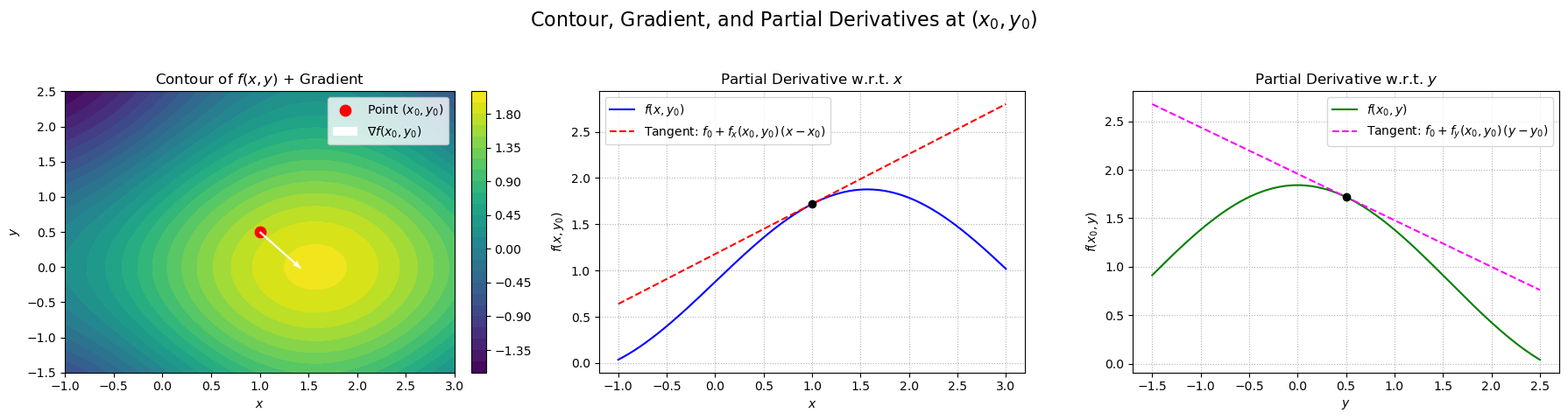
We see in this plot that the gradient \(\nabla f(\mathbf{x})\) points in the direction of steepest ascent from \(\mathbf{x}\). Similarly, the negative gradient \(-\nabla f(\mathbf{x})\) points in the direction of steepest descent from \(\mathbf{x}\).
Theorem (Steepest descent direction)
\(-\nabla f(\mathbf{x})\) points in the direction of steepest descent from \(\mathbf{x}\).
Proof. using the directional derivative and Cauchy–Schwarz:
Let \(f:\mathbb{R}^n\to\mathbb{R}\) be differentiable at a point \(\mathbf{x}\), and let \(\nabla f(\mathbf{x})\) denote its gradient there. For any unit vector \(\mathbf{u}\in\mathbb{R}^n\) (\(\|\mathbf{u}\|=1\)), the directional derivative of \(f\) at \(\mathbf{x}\) in the direction \(\mathbf{u}\) is
We wish to find the direction \(\mathbf{u}\) that minimizes this rate of change (i.e.\ yields the steepest instantaneous decrease). Since \(\mathbf{u}\) is constrained to have unit length, we solve
By the Cauchy–Schwarz inequality,
Moreover, equality holds exactly when \(\mathbf{u}\) is a negative multiple of \(\nabla f(\mathbf{x})\). Imposing \(\|\mathbf{u}\|=1\) gives the unique minimizer
Hence
which is the smallest possible directional derivative over all unit directions. In other words, moving (infinitesimally) in the direction of \(-\nabla f(\mathbf{x})\) decreases \(f\) most rapidly.
We will use this fact frequently when iteratively minimizing a function via gradient descent.
Basic Gradient Descent#
Gradient descent is an optimization algorithm used to minimize a function by iteratively moving in the direction of the steepest descent, as indicated by the negative gradient.
The basic idea is to start at any initial point \(\mathbf{x}_0\) and to iteratively update the current point \(\mathbf{x}_t\) in the following way:
where \(\eta_t\) is the learning rate at iteration \(t\). The learning rate controls the step size of each update.
For now, we can think of the learning rate as a small positive constant \(\eta_t = \eta\) that we simply fix for all iterations. However, note that the choice of learning rate is crucial: too small a value can lead to slow convergence, while too large a value can cause divergence or oscillation around the minimum. Thus, we will discuss learning rate tuning in more detail later.
We also don’t yet have a good way to determine when to stop iterating. For now, we can simply iterate a fixed number of times, or until the change in the function value is small enough. We will discuss more sophisticated stopping criteria later, when we have a better understanding of the properties of minima.
In the following example we show application of the gradient descent algorithm to the function \(f(x,y)=(x-1)^2+2(y-2)^2+\frac{1}{2}\sin(3x)\sin(3y)\), which has a unique global minimum near \((1,2)\). However, we see that small ripples in the function can cause gradient descent to get stuck in local minima.
Show code cell source
import numpy as np
import matplotlib.pyplot as plt

# Define the objective function and its gradient
def f(x, y):
    # A slightly non-convex function: tilted quadratic + sinusoidal ripples
    return (x - 1)**2 + 2*(y - 2)**2 + 0.5 * np.sin(3*x) * np.sin(3*y)

def grad_f(x, y):
    # Partial derivatives
    dfdx = 2*(x - 1) + 1.5 * np.cos(3*x) * np.sin(3*y)
    dfdy = 4*(y - 2) + 1.5 * np.sin(3*x) * np.cos(3*y)
    return np.array([dfdx, dfdy])

# Grid setup
x_vals = np.linspace(-1, 3, 200)
y_vals = np.linspace(-1, 5, 200)
X, Y = np.meshgrid(x_vals, y_vals)
Z = f(X, Y)

# Plot contours
plt.figure(figsize=(8, 6))
contours = plt.contour(X, Y, Z, levels=30, cmap='viridis')
plt.clabel(contours, inline=True, fontsize=8)

# Plot gradient descent vector field (negative gradient)
skip = 15
GX, GY = grad_f(X, Y)
plt.quiver(X[::skip, ::skip], Y[::skip, ::skip],
           -GX[::skip, ::skip], -GY[::skip, ::skip],
           color='gray', alpha=0.6, headwidth=3)

# Simulate gradient descent from several starting points
starts = [(-0.5, 4), (3, -0.5), (2.5, 4.5)]
lr = 0.05
num_steps = 50

for x0, y0 in starts:
    path = np.zeros((num_steps+1, 2))
    path[0] = np.array([x0, y0])
    for i in range(num_steps):
        grad = grad_f(path[i, 0], path[i, 1])
        path[i+1] = path[i] - lr * grad
    plt.plot(path[:, 0], path[:, 1], marker='o', markersize=3,
             label=f"start=({x0:.1f},{y0:.1f})")

# Final touches
plt.title("Contour of $f(x,y)$ with Gradient Descent Paths")
plt.xlabel("$x$")
plt.ylabel("$y$")
plt.legend(loc='upper right')
plt.grid(True)
plt.tight_layout()
plt.show()
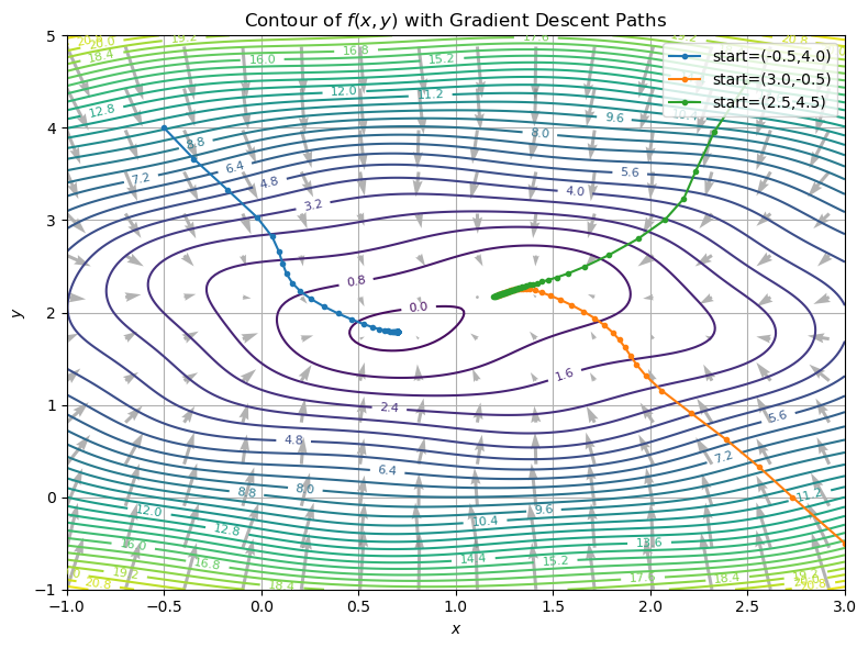
The above figure shows:
Contours of
\[ f(x,y) = (x - 1)^2 + 2(y - 2)^2 + \tfrac12\sin(3x)\sin(3y), \]which has a unique global minimum near \((1,2)\) but small ripples that create nonconvexity.
Gray arrows, indicating the negative gradient direction at each point.
Colored paths, showing gradient‑descent trajectories started from three different initial points. You can see how each path “flows” downhill along the contours, eventually converging to the basin of the global minimum.
Why this helps build intuition:
Contours are level sets of the cost function. Regions where contours are close together indicate steep slopes, while widely spaced contours are flat.
Gradient arrows point in the direction of greatest decrease. Following them leads you toward a local minimum.
Paths from different starts illustrate how gradient descent navigates toward minima and how nonconvex ripples can slow it down or trap it in local basins.
Adjusting the learning rate or initialization changes these trajectories dramatically—showing why step‑size tuning and good initialization matter in practice.