Gradient Descent in Ridge Regression

In this section, we will apply the gradient descent algorithm to the problem of Ridge regression. Ridge regression is a linear regression technique that includes an L2 regularization term to prevent overfitting. The objective function for Ridge regression is given by:

\[ f(\mathbf{w}) = \frac{1}{2}\|\mathbf{y} - \mathbf{X}\mathbf{w}\|^2_2 + \frac{\lambda}{2}\|\mathbf{w}\|^2_2, \]

where \(\mathbf{X}\) is the design matrix, \(\mathbf{y}\) is the response vector, \(\mathbf{w}\) is the weight vector, and \(\lambda\) is the regularization parameter.

The gradient of the objective function with respect to \(\mathbf{w}\) is given by:

\[ \nabla f(\mathbf{w}) = -\mathbf{X}^\top(\mathbf{y} - \mathbf{X}\mathbf{w}) + \lambda\mathbf{w}. \]

We will implement the gradient descent algorithm to minimize this objective function and find the optimal weights \(\mathbf{w}^*\).

import numpy as np

class RidgeRegressionGD:
    def __init__(self, learning_rate=0.01, num_iterations=1000, ridge=0.1):
        self.learning_rate = learning_rate
        self.num_iterations = num_iterations
        self.ridge = ridge

    def mse(self, X, y):
        # Mean Squared Error
        return np.mean((y - self.pred(X)) ** 2)
    
    def loss(self, X, y):
        # Loss function (MSE + Ridge penalty)
        return self.mse(X, y) + self.ridge * np.sum(self.w ** 2)

    def gradient(self, X, y):
        # Gradient of the loss
        return -X.T @ (y - self.pred(X)) / len(y) + self.ridge * self.w

    def fit(self, X, y):
        # Initialize weights
        self.w = np.zeros(X.shape[1])
        
        # Gradient descent loop
        for _ in range(self.num_iterations):   
            self.w -= self.learning_rate * self.gradient(X, y)

    def pred(self, X):
        return X @ self.w

Example usage

We will use the Ridge regression implementation to fit a model to the maximum temperature data from the year 1900. The data is available in the data_train and data_test variables, which contain the training and testing datasets, respectively. We will fit a model based on three tanh basis functions to the data and evaluate its performance using Mean Squared Error (MSE).

The model is given by

\[ \mathbf{y} \approx b + \sum_{i=1}^3 w_i \cdot \phi_i(x; a_i, b_i) \]

where \(\mathbf{y}\) is the temperature, \(x\) is the day of the year.

The tanh basis functions are defined as

\[ \phi_i(x; a_i, b_i) = \tanh(a_i x + b_i) \]

where \(a_i\) and \(b_i\) are the slope and bias hyperparameters, respectively. We will use the following values for the hyperparameters:

\[ a_1 = 0.1, \quad a_2 = 0.2, \quad a_3 = 0.3 \quad \text{and} \quad b_1 = -10, \quad b_2 = -50, \quad b_3 = -100.0 \]

To streamline the implementation, we will collect the hyperparameters for all basis functions \(\phi_i\) in a single matrix \(\mathbf{W}_\phi\):

\[\begin{split} \mathbf{W}_\phi = \begin{pmatrix} a_1 & a_2 & a_3 \\ b_1 & b_2 & b_3 \end{pmatrix} \end{split}\]

Using this notation, we can express the tanh basis functions as:

\[ \boldsymbol{\phi}(x; \mathbf{W}_\phi) = \begin{pmatrix} \tanh(\mathbf{W}_\phi[0,i] x + \mathbf{W}_\phi[1,i]) \end{pmatrix}_{i=1}^3 \]

We implement the tanh basis functions in a class called TanhBasis. The class has two methods: XW and transform. The XW method computes the product of the input data and the weights, while the transform method computes the tanh basis functions.

import numpy as np

class TanhBasis:
    def __init__(self, W):
        self.W = W

    def XW(self, x):
        """Compute the product of the input data and the weights."""
        if len(x.shape) == 1:
            x = x[:, np.newaxis]
        return x @ self.W[:-1] + self.W[-1]

    def transform(self, x):
        """Compute the tanh basis functions."""
        return np.tanh(self.XW(x))

Let’s use the TanhBasis class to fit a Ridge regression model to the maximum temperature data from the year 1900. We will use three tanh basis functions with the specified hyperparameters.

Show code cell source Hide code cell source

import numpy as np
import pandas as pd
import matplotlib.pyplot as plt
YEAR = 1900
def load_weather_data(year = None):
    """
    load data from a weather station in Potsdam
    """

    names = ['station', 'date' , 'type', 'measurement', 'e1','e2', 'E', 'e3']
    data = pd.read_csv('../../datasets/weatherstations/GM000003342.csv', names = names, low_memory=False) # 47876 rows, 8 columns
    # convert the date column to datetime format
    data['date'] = pd.to_datetime(data['date'], format="%Y%m%d") # 47876 unique days
    types = data['type'].unique()

    tmax = data[data['type']=='TMAX'][['date','measurement']] # Maximum temperature (tenths of degrees C), 47876
    tmin = data[data['type']=='TMIN'][['date','measurement']] # Minimum temperature (tenths of degrees C), 47876
    prcp = data[data['type']=='PRCP'][['date','measurement']] # Precipitation (tenths of mm), 47876
    snwd = data[data['type']=='SNWD'][['date','measurement']] # Snow depth (mm), different shape
    tavg = data[data['type']=='TAVG'][['date','measurement']] # average temperature, different shape 1386
    arr = np.array([tmax.measurement.values,tmin.measurement.values, prcp.measurement.values]).T 

    df = pd.DataFrame(arr/10.0, index=tmin.date, columns=['TMAX', 'TMIN', 'PRCP']) # compile data in a dataframe and convert temperatures to degrees C, precipitation to mm

    if year is not None:
        df = df[pd.to_datetime(f'{year}-1-1'):pd.to_datetime(f'{year}-12-31')]
    
    df['days'] = (df.index - df.index.min()).days
    return df

# Load weather data for the year 2000
df = load_weather_data(year = YEAR)

np.random.seed(2)
idx = np.random.permutation(df.shape[0])

idx_train = idx[0:100]
idx_test = idx[100:]

data_train = df.iloc[idx_train]
data_test = df.iloc[idx_test]

N_train = 100

a = np.array([.1, .2, .3])
b = np.array([-10.0,-50.0,-100.0])
W = np.array([a, b])
tanh_basis = TanhBasis(W)

x_train = data_train.days.values[:N_train][:,np.newaxis] * 1.0
X_train = tanh_basis.transform(x_train)
y_train = data_train.TMAX.values[:N_train]

ridge = 0.1     # strength of the L2 penalty in ridge regression
learning_rate = 0.01
num_iterations = 1000
reg = RidgeRegressionGD(ridge=ridge, learning_rate=learning_rate, num_iterations=num_iterations)
reg.fit(X_train, y_train)

x_days = np.arange(366)[:,np.newaxis]
X_days = tanh_basis.transform(x_days)
y_days_pred = reg.pred(X_days)

x_test = data_test.days.values[:,np.newaxis] * 1.0
X_test = tanh_basis.transform(x_test)
y_test = data_test.TMAX.values
y_test_pred = reg.pred(X_test)
print("training MSE : %.4f" % reg.mse(X_train, y_train))
print("test MSE     : %.4f" % reg.mse(X_test, y_test))

fig = plt.figure()
ax = plt.plot(x_train,y_train,'.')
ax = plt.plot(x_test,y_test,'.')
ax = plt.legend(["train MSE = %.2f" % reg.mse(X_train, y_train),"test MSE = %.2f" % reg.mse(X_test, y_test)])
ax = plt.plot(x_days,y_days_pred)
ax = plt.ylim([-27,39])
ax = plt.xlabel("day of the year")
ax = plt.ylabel("Maximum Temperature - degree C")
ax = plt.title("Year : %i        N : %i" % (YEAR, N_train))

training MSE : 29.2677
test MSE     : 32.3784

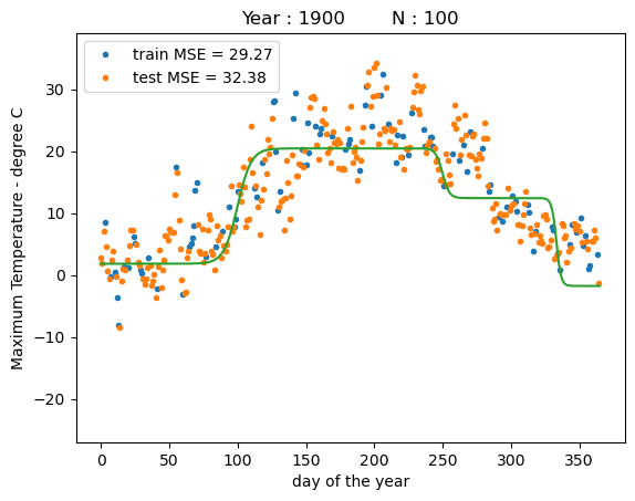
The plot shows that the model fits a model that places three sigmoid basis functions roughly evenly spaced throughout the year. Due to the relatively large slope values the sigmoids look close to step functions. While the model fits the data relatively well, our choice of hyperparameters are far from be optimal.

In the following sections, we will discuss how we can use the gradient descent algorithm to optimize the hyperparameters. However, on order to do so, we will need to introduce the concepts of the Jacobian and the chain rule, that we will discuss in the following sections.