Line Search Methods in Optimization#
So far, we’ve discussed gradient descent, but we haven’t covered how to choose the step size \(\eta_t\).
Line search methods are a family of optimization techniques used to determine how far to move along a given descent direction during iterative optimization like gradient descent.
While the descent direction tells where to go, line search methods answer:
“How far should I go in that direction?”
They are essential for balancing progress (fast convergence) and stability (avoiding overshooting or divergence).
Setup#
Suppose you’re minimizing a differentiable function \(f : \mathbb{R}^n \to \mathbb{R}\), and you’re at a point \(\mathbf{x}_t\) with a descent direction \(\mathbf{d}_t\) (e.g., \(-\nabla f(\mathbf{x}_t)\)).
The line search chooses a step size \(\eta_t > 0\) such that:
The goal is to choose \(\eta_t\) so that it sufficiently decreases the function.
🧠 Types of Line Search Methods#
Line search methods can be broadly categorized into exact and inexact methods.
1. Exact Line Search#
Exact line search reduces the problem to a univariate optimization problem, by creating a 1-dimensional function along the line.
where \(\eta\) is the step size.
It exactly finds the step size \(\eta\) that minimizes the function along the line:
Rare in practice: requires solving a univariate optimization problem exactly.
Used mostly in quadratic problems, where we can find a minimizer analytically, or theory.
2. Backtracking line search#
Backtracking line search is a practical and adaptive method that iteratively shrinks the step size until a sufficient decrease condition is met.
Start with a large step size \(\eta = 1\) and reduce it by a factor \(\beta \in (0, 1)\) until the Armijo condition is met:
The parameter \(c \in (0, 1)\) controls how much decrease is sufficient.
For \(c = 0\), it simply checks if the function value is not increasing compared to current point, which is a very weak condition.
For \(c = 1\) this assumes that \(\phi\) is linear in \(\eta\), which can be seen as a lower bound to \(\phi\).
Intermediate values of \(c\) are used in practice.
The following figure illustrates the Armijo backtracking line search procedure on the 2D quadratic objective function starting at \(\mathbf{x}_0=(0,0)\).
Show code cell source
# Armijo Backtracking Visualization with Exact Line Search

"""
This notebook visualizes how Armijo's sufficient decrease condition affects
step size selection in gradient descent when using backtracking line search,
and compares it to exact line search.

We show:
- The path along the steepest descent direction
- Evaluated candidate steps in backtracking
- The accepted step under Armijo’s condition
- The exact step size minimizing the function along the search direction
"""

import numpy as np
import matplotlib.pyplot as plt

# Define a 2D quadratic objective function and its gradient
def f_2d(x):
    return (x[0] - 2)**2 + 2*(x[1] - 3)**2

def grad_f_2d(x):
    return np.array([2*(x[0] - 2), 4*(x[1] - 3)])

exact_solution = np.array([2, 3])  # Exact solution for the quadratic function

# Define starting point and descent direction
x0 = np.array([0.0, 0.0])
d = -grad_f_2d(x0)  # steepest descent direction

# Line function phi(eta) = f(x0 + eta * d)
def phi(eta):
    return f_2d(x0 + eta * d)

def phi_prime(eta):
    grad = grad_f_2d(x0 + eta * d)
    return np.dot(grad, d)

# Wolfe parameters
c1 = 3e-1
c2 = 0.9
beta = 0.5
eta_vals = np.linspace(-0.1, 0.85, 200)
phi_vals = [phi(a) for a in eta_vals]
armijo_bound = phi(0) + (phi_prime(0) * eta_vals)
armijo_RHS_line = phi(0) + (c1 * phi_prime(0) * eta_vals)

# Backtracking line search candidates
eta_start = 0.8
eta_candidates = [eta_start * beta**i for i in range(3)]
curvature_lhs = [phi_prime(a) for a in eta_candidates]
armijo_lhs = [phi(a) for a in eta_candidates]
curvature_rhs = [c2 * phi_prime(0) for a in eta_candidates]
armijo_rhs = [phi(0) + c1 * a * phi_prime(0) for a in eta_candidates]

# Exact line search: minimize phi analytically (quadratic function)
eta_exact = np.argmin([phi(a) for a in eta_vals])
eta_exact_val = eta_vals[eta_exact]

# Generate 2D contour plot data
x = np.linspace(-1, 4, 400)
y = np.linspace(-1, 10.5, 400)
X, Y = np.meshgrid(x, y)
Z = (X - 2)**2 + 2*(Y - 3)**2

# Path of x(eta) = x0 + eta * d
etas_path = np.linspace(0, 1.5, 50)
path = np.array([x0 + a * d for a in etas_path])

# Create subplots
fig, (ax1, ax2) = plt.subplots(1, 2, figsize=(14, 6))

# Plot 2D contour and line search path
contour = ax1.contour(X, Y, Z, levels=30, cmap='viridis')
ax1.scatter(exact_solution[0], exact_solution[1], color='black', label=r'minimum of $f$')
ax1.plot(path[:, 0], path[:, 1], color='red', label='Line search path')
ax1.scatter(*x0, color='blue', label=r'Start $\mathbf{x}_0$')
ax1.scatter(*(x0 + eta_candidates[0] * d), color='red', label=r'rejected $\eta=0.8$')
ax1.scatter(*(x0 + eta_candidates[1] * d), color='red', label=r'rejected $\eta=0.4$')
ax1.scatter(*(x0 + eta_candidates[-1] * d), color='green', label=r'accepted $\eta=0.2$')
ax1.scatter(*(x0 + eta_exact_val * d), color='black', marker='x', s=80, label=r'exact line search step $\eta^*$')
ax1.set_title("2D Contour Plot of $f(x)$ and Search Direction")
ax1.set_xlabel("x")
ax1.set_ylabel("y")
ax1.set_xlim(-1, 4)
ax1.set_ylim(-1, 10.5)
ax1.legend()

# Plot phi(eta) along search direction
ax2.plot(eta_vals, phi_vals, label=r'$\psi(\eta) = f(x_0 + \eta d)$', color='red')
ax2.plot(eta_vals, armijo_bound, '--', label='linear approximation', color='gray')
ax2.plot(eta_vals[eta_vals >= 0], armijo_RHS_line[eta_vals >= 0], '--', label=('Armijo RHS, $c=%.2f$' % c1), color='purple')
ax2.scatter(0, phi(0), color='blue', label=r'$\psi(0)$', zorder=5)
ax2.scatter(eta_candidates[:-1], armijo_lhs[:-1], color='red', label='rejected evaluations')
ax2.scatter(eta_candidates[-1], armijo_lhs[-1], color='green', label='accepted step')
ax2.scatter(eta_exact_val, phi(eta_exact_val), color='black', marker='x', s=80, label=r'exact line search $\eta^*$')
ax2.set_title("1D Function Along Search Direction")
ax2.set_xlabel(r'$\eta$')
ax2.set_ylabel(r'$\psi(\eta)$')
ax2.legend()
ax2.grid(True)
ax2.set_xlim(-0.1, 0.85)
ax2.set_ylim(-20, 100)

plt.tight_layout()
plt.show()
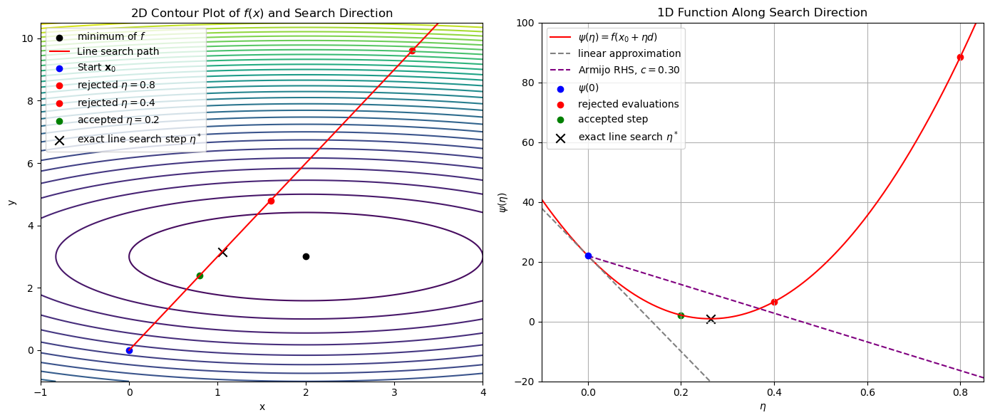
The left panel shows the level sets (contours) of the function together with the path along the steepest descent direction from the starting point \(\mathbf{x}_0 = (0, 0)\). Three candidate steps along this direction are evaluated:
The two red dots correspond to candidate step sizes \(\eta = 0.8\) and \(\eta = 0.4\), which are rejected by the Armijo condition.
The green dot at \(\eta = 0.2\) represents the first candidate that satisfies the Armijo condition and is therefore accepted.
The right panel shows the function \(\psi(\eta) = f(\mathbf{x}_0 + \eta \mathbf{d})\), which is the value of the objective function along the search direction.
The red curve plots \(\psi(\eta)\).
The gray dashed line is the first-order linear approximation \(\psi(0) + \psi'(0)\eta\), while the purple dashed line is the Armijo threshold with parameter \(c_1 = 0.3\).
The red and green points mark the same backtracking evaluations as in the left panel, visualized now as function values.
The region below the purple line represents all step sizes that satisfy the Armijo condition. The accepted step \(\eta = 0.2\) is the first point along this curve to fall in this region.
Implementation of Backtracking Line Search#
In the following, we will implement a class for gradient descent with the backtracking line search method, which will be used in the next sections to optimize the objective function. We also add a stopping criterion based on the first order optimality condition that checks the norm of the gradient vector.
class GradientDescentArmijo:
    def __init__(self, f, grad_f, x0, c1=1.0, beta=0.5, tol=1e-6, max_iter=10000, eta0=1.0, max_iter_backtrack=100):
        self.f = f
        self.eta0 = eta0
        self.grad_f = grad_f
        self.x = x0
        self.c1 = c1
        self.beta = beta
        self.tol = tol
        self.max_iter = max_iter
        self.max_iter_backtrack = max_iter_backtrack
        self.path = [x0.copy()]
        self.etas = []
        self.f_path = []
        self.grad_path = []
        self.optimizer = None

    def backtracking_line_search(self, d, f0, grad_f0):
        eta = self.eta0
        for _ in range(self.max_iter_backtrack):
            if self.f(self.x + eta * d) <= f0 + self.c1 * eta * np.dot(grad_f0, d):
                return eta
            eta *= self.beta
        return -1.0 # if no step is found

    def run(self):
        for _ in range(self.max_iter):
            grad = self.grad_f(self.x)
            f = self.f(self.x)
            self.f_path.append(f)
            self.grad_path.append(grad)
            if np.linalg.norm(grad) < self.tol:
                break
            d = -grad
            eta = self.backtracking_line_search(d, f, grad)
            if eta <= 0.0:
                break
            self.x = self.x + eta * d
            self.path.append(self.x.copy())
            self.etas.append(eta)
        return self.x
We also have to adapt our ridge regression implementation to use the GradientDescentArmijo class in the fit method.
class BasisFunctionRidgeRegressionGD:
    def __init__(self, basis_function, ridge=0.1, ridge_basis=0.1):
        self.basis_function = basis_function
        self.ridge = ridge
        self.ridge_basis = ridge_basis
        self.w = None

    def mse(self, X, y):
        residuals = (y - self.pred(X))
        return np.mean(residuals*residuals)

    def d_loss_d_Phi(self, Phi, y):
        N = Phi.shape[0]
        if self.w is None:
            self.w = np.zeros(Phi.shape[1])
        residuals = (y - Phi @ self.w)
        return -residuals[:,np.newaxis] * self.w[np.newaxis,:] / N

    def loss(self, X, y):
        Phi = self.basis_function.transform(X)
        residuals = (y - Phi @ self.w)
        mse = np.mean(residuals*residuals)
        L = 0.5*mse + 0.5*self.ridge*np.sum(self.w**2)
        L += 0.5*self.ridge_basis*np.sum(self.basis_function.W**2)
        return L

    def gradient_w(self, X, y):
        return -(self.basis_function.transform(X).T @ (y - self.pred(X))) / len(y) + self.ridge * self.w

    def gradient_basis_function(self, X, y):
        return -self.w[np.newaxis,:] * (y - self.pred(X))[:,np.newaxis] / len(y)

    def gradient_basis_function_W(self, X, y):
        grad_loss_bf = self.gradient_basis_function(X, y)
        jacobian_phi = self.basis_function.jacobian(X)
        res = grad_loss_bf[:, None, :] * jacobian_phi
        gW = res.sum(0)
        gW += self.ridge_basis * self.basis_function.W
        return gW

    def fit(self, X, y, c1=1e-4, beta=0.5, tol=1e-6, max_iter=100, eta0=1.0):
        Phi = self.basis_function.transform(X)
        self.w = np.zeros(Phi.shape[1])

        def loss_W(W_flat):
            self.basis_function.W = W_flat.reshape(self.basis_function.W.shape)
            return self.loss(X, y)

        def grad_W(W_flat):
            self.basis_function.W = W_flat.reshape(self.basis_function.W.shape)
            return self.gradient_basis_function_W(X, y).flatten()

        self.optimizer = GradientDescentArmijo(f=loss_W, grad_f=grad_W, x0=self.basis_function.W.flatten(),
                                          c1=c1, beta=beta, tol=tol, max_iter=max_iter, eta0=eta0)
        W_optimized = self.optimizer.run().reshape(self.basis_function.W.shape)
        self.basis_function.W = W_optimized

        # update w using closed form ridge solution
        Phi = self.basis_function.transform(X)
        self.w = np.linalg.solve(Phi.T @ Phi + self.ridge * np.eye(Phi.shape[1]), Phi.T @ y)

    def pred(self, X):
        Phi = self.basis_function.transform(X)
        if self.w is None:
            self.w = np.zeros(Phi.shape[1])
        return Phi @ self.w

    def numerical_grad_W(self, X, y, eps=1e-7):
        W = self.basis_function.W
        num_grad = np.zeros_like(W)
        it = np.nditer(W, flags=['multi_index'], op_flags=['readwrite'])
        while not it.finished:
            idx = it.multi_index
            orig = W[idx]
            W[idx] = orig + eps
            loss_plus = self.loss(X, y)
            W[idx] = orig - eps
            loss_minus = self.loss(X, y)
            num_grad[idx] = (loss_plus - loss_minus) / (2*eps)
            W[idx] = orig
            it.iternext()
        return num_grad
Let’s test the implementation with our temperature prediction example. The basis function class TanhBasis does not require any changes.
Show code cell source
import numpy as np
class TanhBasis:
    def __init__(self, W):
        self.W = W.copy()

    def Z(self, X):
        if len(X.shape) == 1:
            X = X[:, np.newaxis]
        return X @ self.W[:-1] + self.W[-1]

    def transform(self, X):
        return np.tanh(self.Z(X))

    def jacobian(self, X):
        if len(X.shape) == 1:
            X = X[:, np.newaxis]
        dZ_dW = np.hstack((X, np.ones((X.shape[0], 1))))
        dPhi_dz = (1 - np.tanh(self.Z(X))**2)
        return dZ_dW[:,:,np.newaxis] * dPhi_dz[:,np.newaxis,:]

    def numerical_jacobian(self, X, eps=1e-6):
        original_W = self.W.copy()
        N, D = X.shape
        K = self.W.shape[1]
        num_J = np.zeros((N, D+1, K))
        for d in range(D+1):
            for k in range(K):
                self.W = original_W.copy()
                self.W[d, k] += eps
                phi_plus = self.transform(X)
                self.W = original_W.copy()
                self.W[d, k] -= eps
                phi_minus = self.transform(X)
                num_J[:, d, k] = (phi_plus[:, k] - phi_minus[:, k]) / (2 * eps)
        self.W = original_W
        return num_J

import pandas as pd
import matplotlib.pyplot as plt
YEAR = 1900
def load_weather_data(year = None):
    """
    load data from a weather station in Potsdam
    """

    names = ['station', 'date' , 'type', 'measurement', 'e1','e2', 'E', 'e3']
    data = pd.read_csv('../../datasets/weatherstations/GM000003342.csv', names = names, low_memory=False) # 47876 rows, 8 columns
    # convert the date column to datetime format
    data['date'] = pd.to_datetime(data['date'], format="%Y%m%d") # 47876 unique days
    types = data['type'].unique()

    tmax = data[data['type']=='TMAX'][['date','measurement']] # Maximum temperature (tenths of degrees C), 47876
    tmin = data[data['type']=='TMIN'][['date','measurement']] # Minimum temperature (tenths of degrees C), 47876
    prcp = data[data['type']=='PRCP'][['date','measurement']] # Precipitation (tenths of mm), 47876
    snwd = data[data['type']=='SNWD'][['date','measurement']] # Snow depth (mm), different shape
    tavg = data[data['type']=='TAVG'][['date','measurement']] # average temperature, different shape 1386
    arr = np.array([tmax.measurement.values,tmin.measurement.values, prcp.measurement.values]).T

    df = pd.DataFrame(arr/10.0, index=tmin.date, columns=['TMAX', 'TMIN', 'PRCP']) # compile data in a dataframe and convert temperatures to degrees C, precipitation to mm

    if year is not None:
        df = df[pd.to_datetime(f'{year}-1-1'):pd.to_datetime(f'{year}-12-31')]

    df['days'] = (df.index - df.index.min()).days
    return df

# Load weather data for the year 2000
df = load_weather_data(year = YEAR)

np.random.seed(2)
idx = np.random.permutation(df.shape[0])

N_train = 100

idx_train = idx[0:N_train]
idx_test = idx[N_train:]

data_train = df.iloc[idx_train]
data_test = df.iloc[idx_test]

a = np.array([.1, .2, .3])
b = np.array([-10.0,-50.0,-100.0])
W = np.array([a, b])

# tanh_basis = TanhBasis(W)
tanh_basis = TanhBasis(W)

ridge = 0.1     # strength of the L2 penalty in ridge regression
ridge_basis = 0.1     # strength of the L2 penalty on the parameters of the basis function

x_train = data_train.days.values[:N_train][:,np.newaxis] * 1.0
# X_train = tanh_basis(x_train, a, b)
y_train = data_train.TMAX.values[:N_train]

reg = BasisFunctionRidgeRegressionGD(basis_function=tanh_basis,ridge=ridge, ridge_basis=ridge_basis)
reg.fit(x_train, y_train, c1=0.999, beta=0.1, tol=1e-5, max_iter=2000, eta0=0.1)

x_days = np.arange(366)[:,np.newaxis]
y_days_pred = reg.pred(x_days)

x_test = data_test.days.values[:,np.newaxis] * 1.0
y_test = data_test.TMAX.values
y_test_pred = reg.pred(x_test)
print("training MSE : %.4f" % reg.mse(x_train, y_train))
print("test MSE     : %.4f" % reg.mse(x_test, y_test))


fig = plt.figure()
ax = plt.plot(x_train,y_train,'.')
ax = plt.plot(x_test,y_test,'.')
ax = plt.legend(["train MSE = %.2f" % reg.mse(x_train, y_train),"test MSE = %.2f" % reg.mse(x_test, y_test)])
ax = plt.plot(x_days,y_days_pred)
ax = plt.ylim([-27,39])
ax = plt.xlabel("day of the year")
ax = plt.ylabel("Maximum Temperature - degree C")
ax = plt.title("Year : %i        N : %i" % (YEAR, N_train))
training MSE : 17.9200
test MSE     : 20.8156
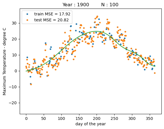
We can see that the model is able to fit the training data even better than using vanilla gradient descent without line search. The resulting function now has a much smoother shape. However, we see that on the test data the model yields a similar performance as before.