Mean value theorem#
We discuss the Mean Value Theorem (MVT) in both single and multiple variables. The MVT is a fundamental theorem in calculus that provides a connection between the derivative of a function and its average rate of change over an interval.
The MVT will help us understand the gradient descent algorithm and its convergence properties. It will also be a cornerstone for the Taylor expansion, which is a powerful tool for approximating functions and the basis of second order optimization algorithms.
Mean value theorem in 1 variable#
The Mean Value Theorem (MVT) is one of the cornerstones of single‐variable calculus. Informally, it says that for any smooth curve connecting two points, there is at least one point in between where the instantaneous slope (the derivative) matches the average slope over the whole interval. The MVT is a special case of the Fundamental Theorem of Calculus that links the derivative of a function to its integral.
Theorem (Mean value theorem)
Let \(f:[a,b]\to\mathbb{R}\) be a continuous function on the closed interval \([a,b]\), and differentiable on the open interval \((a,b)\), where \(a\neq b\).
Then there exists some \(c \in (a,b)\) such that
In other words, the tangent line at \(x=c\) is exactly parallel to the secant line joining \((a,f(a))\) and \((b,f(b))\). A proof of the MVT is provided in the Appendix.
Below, we illustrate the MVT for the cubic \(f(x)=x + x^3\) on the intervals \([0.5,2.0]\) and \([-1.5,1.5]\).
Show code cell source
import numpy as np
import matplotlib.pyplot as plt

# Define the function and its derivative
def f(x):   return x**3 + x
def df(x):  return 3 * x**2 + 1

# Intervals for demonstration
intervals = [
    (0.5, 2.0, "Interval [0.5, 2.0]"),
    (-1.5, 1.5, "Interval [-1.5, 1.5] (inflection)")
]

# Prepare figure with two subplots
fig, axes = plt.subplots(1, 2, figsize=(14, 7), sharey=True)

x_all = np.linspace(-1.7, 2.5, 400)

for ax, (a, b, title) in zip(axes, intervals):
    # Compute secant slope
    m = (f(b) - f(a)) / (b - a)
    # Solve f'(c) = m => 3 c^2 + 1 = m => c = ±sqrt( (m-1)/3 )
    cs = []
    sol = np.sqrt((m-1) / 3)
    for c in [ sol, -sol]:
        if a < c < b:
            cs.append(c)

    # Plot the true function
    ax.plot(x_all, f(x_all), label='$f(x)=x^3$', color='gold', linewidth=2)
    # Plot the secant line
    secant = f(a) + m * (x_all - a)
    ax.plot(x_all, secant, '--', label=f'Secant (slope={m:.2f})', color='orange')

    # Plot tangent(s) at each c
    for c in cs:
        tangent = f(c) + m * (x_all - c)
        ax.plot(x_all, tangent, ':', label=f'Tangent at c={c:.2f}', linewidth=2)
        ax.scatter([c], [f(c)], color='red', s=80)

    # Mark endpoints
    ax.scatter([a, b], [f(a), f(b)], color='blue', s=80)
    ax.set_ylim([-7,15])
    ax.set_xlim([-1.7, 2.5])
    ax.set_title(title)
    ax.set_xlabel('x')
    ax.grid(True)
    ax.legend()

axes[0].set_ylabel('f(x)')
plt.suptitle('Mean Value Theorem: Secant vs Tangent—Including Inflection Example')
plt.tight_layout(rect=[0, 0.03, 1, 0.95])
plt.show()
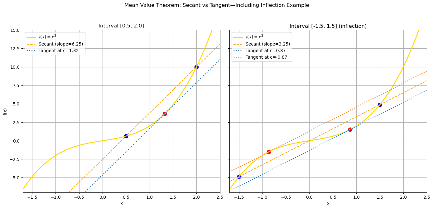
We observe that for the interval \([0.5,2.0]\), the secant line (orange dashed) and the tangent line (red dotted) at \(x=c\) are parallel, as expected. For the interval \([-1.5,1.5]\), we see that the secant line is parallel to the tangent line at two different points \(c_1\) and \(c_2\). The existence of multiple different points with parallel tangent lines is consistent with the MVT, as the function \(f\) can have inflection points where the second derivative changes its sign within the interval, such as \(x=0\) in our example.
Mean Value Theorem for real-valued Functions in Several Variables#
The Mean Value Theorem can be extended to real-valued functions of several variables.
Corollary (Mean value theorem for several variables)
If \(f:\mathbf{R}^n\to\mathbf{R}\) be continuously differentiable, then for any two points \(\mathbf{x},\mathbf{y}\in\mathbf{R}^n\), there exists a point \(\mathbf{z}\) on the line segment \(\mathbf{z}(t)=(1-t)\mathbf{x}+t\mathbf{y}\), \(t\in[0,1]\), such that
Before we prove this corollary, we will first illustrate it with a simple example.
Show code cell source
import numpy as np
import matplotlib.pyplot as plt

# Define multivariate function and its gradient
def f2d(X):
    # X: array of shape (n_points, 2)
    return np.sum(X**2, axis=1)

def grad_f2d(x):
    # x: array shape (2,)
    return 2 * x

# Choose two points in R^2
x = np.array([-1.0, 0.5])
y = np.array([2.0, -1.0])
z = 0.5 * (x + y)  # midpoint c=0.5

# Direction vector and function values
d = y - x
f_x = f2d(x[np.newaxis, :])[0]
f_y = f2d(y[np.newaxis, :])[0]

# Define g(t) and its derivative g'(t)
def g(t):
    X_t = (1 - t)[:, None] * x + t[:, None] * y
    return f2d(X_t)

def g_prime(t):
    X_t = (1 - t)[:, None] * x + t[:, None] * y
    grads = np.array([grad_f2d(pt) for pt in X_t])
    return np.einsum('ij,j->i', grads, d)

# Sample t values
t_vals = np.linspace(0, 1, 200)
g_vals = g(t_vals)
secant_line = f_x + (f_y - f_x) * t_vals
tangent_line = f2d(z[np.newaxis, :])[0] + (2*z).dot(d) * (t_vals - 0.5)  # slope = g'(0.5)

# Plotting
fig, (ax1, ax2) = plt.subplots(1, 2, figsize=(14, 6))

# Left: contour in R^2
xx, yy = np.meshgrid(np.linspace(-2, 3, 200), np.linspace(-2, 2, 200))
XY = np.stack([xx.ravel(), yy.ravel()], axis=1)
zz = f2d(XY).reshape(xx.shape)
contours = ax1.contour(xx, yy, zz, levels=20, cmap='viridis')
ax1.clabel(contours, inline=True, fontsize=8)
ax1.scatter(*x, color='blue', label='x', s=80)
ax1.scatter(*y, color='green', label='y', s=80)
ax1.scatter(*z, color='red', label='z = midpoint', s=80)

# Gradient arrow at z
grad_z = grad_f2d(z)
ax1.arrow(z[0], z[1], grad_z[0], grad_z[1],
          head_width=0.1, head_length=0.1, color='red', label='∇f(z)')
# Direction arrow (y-x) at z
ax1.arrow(x[0], x[1], d[0], d[1],
          head_width=0.1, head_length=0.1, color='orange', label='y - x', alpha=0.5)

ax1.set_title('Contour of $f(x_1,x_2)=x_1^2+x_2^2$\nwith points and vectors')
ax1.set_xlabel('$x_1$')
ax1.set_ylabel('$x_2$')
ax1.legend()
ax1.grid(True)

# Right: g(t) vs t
ax2.plot(t_vals, g_vals, label=r'$g(t)=f((1-t)\mathbf{x}+t\mathbf{y})$')
ax2.plot(t_vals, secant_line, '--', label='Secant line')
ax2.plot(t_vals, tangent_line, ':', label='Tangent at $t=0.5$')
ax2.scatter([0, 1, 0.5], [f_x, f_y, f2d(z[np.newaxis, :])[0]],
            color=['blue', 'green', 'red'], s=80)

ax2.set_title('1D View: $g(t)$, Secant vs. Tangent at $c=0.5$')
ax2.set_xlabel('t')
ax2.set_ylabel('g(t)')
ax2.legend()
ax2.grid(True)

plt.tight_layout()
plt.show()
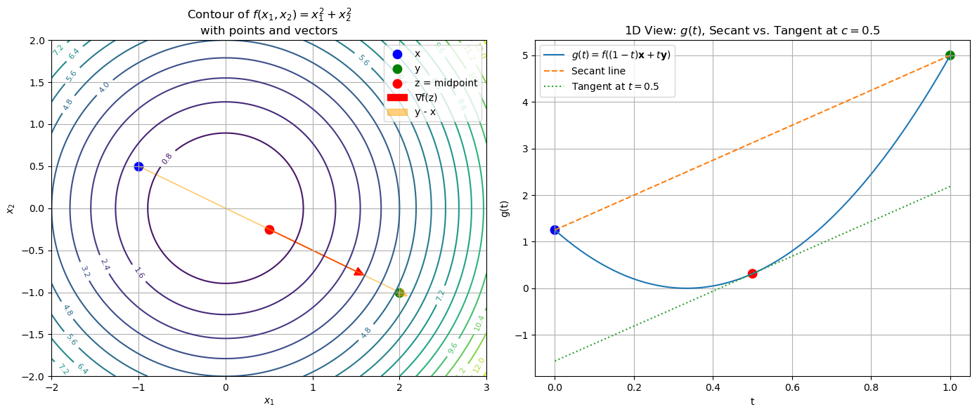
The left plot shows the contour of the function \(f(x_1,x_2)=x_1^2+x_2^2\) in \(\mathbb{R}^2\), with the points \(\mathbf{x}\), \(\mathbf{y}\), and their midpoint \(\mathbf{z}\) marked. The right plot shows the function \(g(t)=f\bigl((1-t)\mathbf{x} + t\,\mathbf{y}\bigr)\) as a function of \(t\). In the right plot, the secant line (dashed) connects \(g(0)=f(\mathbf{x})\) and \(g(1)=f(\mathbf{y})\), while the tangent line (dotted) at \(t=0.5\) has the same slope as the secant line.
Proof. Let \(f:\mathbf{R}^n\to\mathbf{R}\) be continuously differentiable, and pick any two points \(\mathbf{x},\mathbf{y}\in\mathbf{R}^n\). We want to relate
to the gradient of \(f\).
To do so, we need to parameterize the line segment: Define
Then \(\mathbf{z}(0)=\mathbf{x}\) and \(\mathbf{z}(1)=\mathbf{y}\).
Next, we build a one‐variable function on the line segment.
Consider
Since \(\mathbf{z}\) is affine and \(f\) is differentiable, \(g\) is differentiable on \([0,1]\).
This definition allows us to apply the 1D MVT to \(g\).
By the single‐variable Mean Value Theorem, there exists some \(c\in(0,1)\) such that
But \(g(1)=f(\mathbf{y})\) and \(g(0)=f(\mathbf{x})\), so
We need to compute \(g'(c)\). Remember that \(g(t)=f\bigl(\mathbf{z}(t)\bigr)\), so we can apply the chain rule:
Here \(\nabla f\) is the gradient of \(f\) at \(\mathbf{z}(t)\), and \(\mathbf{z}'(t)\) is the vector of partial derivatives of \(\mathbf{z}\) at \(t\):
Hence
In particular, at \(t=c\):
If we combine the previous steps, we have
Finally, we can derive a Lipschitz bound via the Cauchy–Schwarz inequality.
Corollary (Lipschitz continuity)
If \(f:\mathbf{R}^n\to\mathbf{R}\) is continuously differentiable, then for any two points \(\mathbf{x},\mathbf{y}\in\mathbf{R}^n\), there exists a point \(\mathbf{z}\) on the line segment \(\mathbf{z}(t)=(1-t)\mathbf{x}+t\mathbf{y}\), \(t\in[0,1]\), such that
If moreover \(\|\nabla f(\mathbf{z})\|\le L\) everywhere along the segment, then
In the latter case, we say that \(f\) is Lipschitz continuous with constant \(L\). In other words, the function \(f\) does not change too rapidly. This is a very useful property, as it allows us to control the difference in function values based on the distance between points in the domain. This is particularly important in optimization, where we want to ensure that small changes in the input lead to small changes in the output, a property that is often desired for convergence of algorithms.
Proof. Lipschitz continuity
Let \(f:\mathbf{R}^n\to\mathbf{R}\) be continuously differentiable, and pick any two points \(\mathbf{x},\mathbf{y}\in\mathbf{R}^n\).
We have already shown that there exists a point \(\mathbf{z}(c)=(1-c)\mathbf{x}+c\mathbf{y}\) on the line segment between \(\mathbf{x}\) and \(\mathbf{y}\) such that
The first ressult follows from the Cauchy–Schwarz inequality:
If we assume that \(\|\nabla f(\mathbf{z})\|\le L\) everywhere along the segment, then we can bound the right-hand side by \(L\,\|\mathbf{y}-\mathbf{x}\|_2\) to get the second result:
This shows that \(f\) is Lipschitz continuous with constant \(L\).
Mean Value Theorem for Vector-Valued Functions#
The standard Mean Value Theorem (MVT) holds for real-valued functions \(f:\mathbb{R} \to \mathbb{R}\). However, for vector-valued functions \(\mathbf{f}:\mathbb{R}^n \to \mathbb{R}^m\), a direct analog generally does not exist. This is because applying the mean value theorem componentwise results in different intermediate points \(t_i\) for each component, making it impossible, in general, to find a single point that satisfies the theorem for all components simultaneously.
Instead, a useful generalized form involving integrals (the Jacobian Lemma) can be employed.
Let \(\mathbf{f}:\mathbb{R}^n\to\mathbb{R}^m\) be continuously differentiable, and let \(\mathbf{x},\mathbf{h}\in\mathbb{R}^n\). Then, there exists an integral-based formula involving the Jacobian matrix \(\mathbf{J}_{\mathbf{f}}\), defined as:
The lemma is stated rigorously as follows:
Theorem (Jacobian Lemma (Generalized Vector-Valued MVT))
Let \(\mathbf{f}:\mathbb{R}^n\to\mathbb{R}^m\) be continuously differentiable, and let \(\mathbf{x},\mathbf{h}\in\mathbb{R}^n\).
Then:
where the integral of the Jacobian matrix is understood componentwise.
Note that the comoponent-wise integral of Jacobian yields an \(m\times n\) matrix. Thus, the right-hand side of the equation is a matrix-vector product, yielding a vector in \(\mathbb{R}^m\).
Proof. Jacobian Lemma
We will prove the Jacobian lemma using the chain rule and the Second Fundamental Theorem of Calculus. Let \(\mathbf{f}:\mathbb{R}^n\to\mathbb{R}^m\) be continuously differentiable, and let \(\mathbf{x},\mathbf{h}\in\mathbb{R}^n\).
We will need two ingredients:
Ingredient 1: Define the auxiliary function.
We define the auxiliary function \(\mathbf{g}(t)\) by:
Then \(\mathbf{g}\) is differentiable and by the chain rule, we get the vector-valued derivative:
Ingredient 2: Apply the Fundamental Theorem of Calculus.
By the Second Fundamental Theorem of Calculus that states that the difference of a function over an interval \([a,b]\) can be expressed as the integral of its derivative over that interval, we have:
Putting it together:
Our goal is to express the difference \(\mathbf{f}(\mathbf{x}+\mathbf{h}) - \mathbf{f}(\mathbf{x})\) in terms of the integral of the Jacobian matrix.
We can do this by substituting the definition of \(\mathbf{g}(t)\) in ingredient 1, the difference if \(\mathbf{f}(\mathbf{x}+\mathbf{h})\) and \(\mathbf{f}(\mathbf{x})\) can be expressed as the change in \(\mathbf{g}\) over the interval \([0,1]\):
Using ingriedient 2, we can express this difference in the values of \(\mathbf{g}\) at points \(0\) and \(1\) as the integral of its derivative over the interval \([0,1]\):
Plugging in the expression for \(\mathbf{g}'(t)\) derived above gives us:
Since \(\mathbf{h}\) is constant, we factor it out to the right to obtain the desired result:
This proves the Jacobian Lemma. ◻
The Jacobian lemma is particularly useful in optimization and numerical analysis, as it allows us to approximate the change in a vector-valued function using the average of its Jacobian over the interval. This is especially important when dealing with high-dimensional spaces, where direct computation of the function’s value can be expensive.
Summary#
In summary, the Mean Value Theorem and its generalizations, such as the Jacobian lemma, are essential tools in calculus and optimization. They provide a framework for understanding the behavior of functions and their derivatives.
Next, we will use the Mean Value Theorem and the Jacobian lemma to analyze optimality conditions and convergence properties of the gradient descent algorithm.