Ridge Regression as a Quadratic Optimization Problem#
So far, we have optimized ridge regression using the gradient descent algorithm. However, the first order condition tells us that at the minimum of the objective function, the gradient should vanish. We will use this knowledge to derive an analytical solution to the weights in ridge regression. We will show that Ridge Regression belongs to the set of quadratic Optimization Problems and will show how to solve quadratic optimization problems analytically.
Ride Regression#
The objective function for Ridge regression is given by:
where \(\mathbf{X}\) is the design matrix, \(\mathbf{y}\) is the response vector, \(\mathbf{w}\) is the weight vector, and \(\lambda\) is the regularization parameter.
To derive the analytical solution for Ridge regression, we proceed by setting the gradient of the objective function to zero, since at the minimum, the gradient must vanish.
The gradient of the objective function with respect to \(\mathbf{w}\) is given by:
Step 1: Set the gradient to zero
Step 2: Expand the expression
Step 3: Move \(-\mathbf{X}^\top\mathbf{y}\) to the other side
Step 4: Factor out \(\mathbf{w}\)
Here, \(\mathbf{I}\) is the identity matrix of the same dimension as \(\mathbf{X}^\top\mathbf{X}\).
Step 5: Solve for \(\mathbf{w}\)
Assuming \((\mathbf{X}^\top\mathbf{X} + \lambda \mathbf{I})\) is invertible (which it is for \(\lambda > 0\)):
This is the closed-form (analytical) solution for the Ridge regression weights.
Let’s implement the closed form solution. It significantly simplifies the implementation compared to our version using gradient descent.
import numpy as np

class RidgeRegression:
    def __init__(self, ridge=0.1):
        self.ridge = ridge

    def mse(self, X, y):
        # Mean Squared Error
        return np.mean((y - self.pred(X)) ** 2)

    def loss(self, X, y):
        # Loss function (MSE + Ridge penalty)
        return self.mse(X, y) + self.ridge * np.sum(self.w ** 2)

    def fit(self, X, y):
        # Compute the closed form Solution for the weights
        XX = X.T @ X + self.ridge * np.eye(X.shape[1])
        Xy = X.T @ y
        self.w = np.linalg.inv(XX) @ Xy

    def pred(self, X):
        return X @ self.w
Example usage#
We will use the Ridge regression implementation to fit a model to the maximum temperature data from the year 1900. We will fit a model based on three tanh basis functions with the fixed parameters defined before, without optimizing over the basis functions.
The model is given by
where \(\mathbf{y}\) is the temperature, \(x\) is the day of the year.
The tanh basis functions are defined as
where \(a_i\) and \(b_i\) are the slope and bias hyperparameters, respectively. We will use the following values for the hyperparameters:
Show code cell source
import numpy as np
import pandas as pd
import matplotlib.pyplot as plt

import numpy as np

class TanhBasis:
    def __init__(self, W):
        self.W = W

    def XW(self, x):
        """Compute the product of the input data and the weights."""
        if len(x.shape) == 1:
            x = x[:, np.newaxis]
        return x @ self.W[:-1] + self.W[-1]

    def transform(self, x):
        """Compute the tanh basis functions."""
        return np.tanh(self.XW(x))

YEAR = 1900
def load_weather_data(year = None):
    """
    load data from a weather station in Potsdam
    """

    names = ['station', 'date' , 'type', 'measurement', 'e1','e2', 'E', 'e3']
    data = pd.read_csv('../../datasets/weatherstations/GM000003342.csv', names = names, low_memory=False) # 47876 rows, 8 columns
    # convert the date column to datetime format
    data['date'] = pd.to_datetime(data['date'], format="%Y%m%d") # 47876 unique days
    types = data['type'].unique()

    tmax = data[data['type']=='TMAX'][['date','measurement']] # Maximum temperature (tenths of degrees C), 47876
    tmin = data[data['type']=='TMIN'][['date','measurement']] # Minimum temperature (tenths of degrees C), 47876
    prcp = data[data['type']=='PRCP'][['date','measurement']] # Precipitation (tenths of mm), 47876
    snwd = data[data['type']=='SNWD'][['date','measurement']] # Snow depth (mm), different shape
    tavg = data[data['type']=='TAVG'][['date','measurement']] # average temperature, different shape 1386
    arr = np.array([tmax.measurement.values,tmin.measurement.values, prcp.measurement.values]).T

    df = pd.DataFrame(arr/10.0, index=tmin.date, columns=['TMAX', 'TMIN', 'PRCP']) # compile data in a dataframe and convert temperatures to degrees C, precipitation to mm

    if year is not None:
        df = df[pd.to_datetime(f'{year}-1-1'):pd.to_datetime(f'{year}-12-31')]

    df['days'] = (df.index - df.index.min()).days
    return df

# Load weather data for the year 2000
df = load_weather_data(year = YEAR)

np.random.seed(2)
idx = np.random.permutation(df.shape[0])

idx_train = idx[0:100]
idx_test = idx[100:]

data_train = df.iloc[idx_train]
data_test = df.iloc[idx_test]

N_train = 100

a = np.array([.1, .2, .3])
b = np.array([-10.0,-50.0,-100.0])
W = np.array([a, b])
tanh_basis = TanhBasis(W)

x_train = data_train.days.values[:N_train][:,np.newaxis] * 1.0
X_train = tanh_basis.transform(x_train)
y_train = data_train.TMAX.values[:N_train]

ridge = 0.1     # strength of the L2 penalty in ridge regression
reg = RidgeRegression(ridge=ridge)
reg.fit(X_train, y_train)

x_days = np.arange(366)[:,np.newaxis]
X_days = tanh_basis.transform(x_days)
y_days_pred = reg.pred(X_days)

x_test = data_test.days.values[:,np.newaxis] * 1.0
X_test = tanh_basis.transform(x_test)
y_test = data_test.TMAX.values
y_test_pred = reg.pred(X_test)
print("training MSE : %.4f" % reg.mse(X_train, y_train))
print("test MSE     : %.4f" % reg.mse(X_test, y_test))

fig = plt.figure()
ax = plt.plot(x_train,y_train,'.')
ax = plt.plot(x_test,y_test,'.')
ax = plt.legend(["train MSE = %.2f" % reg.mse(X_train, y_train),"test MSE = %.2f" % reg.mse(X_test, y_test)])
ax = plt.plot(x_days,y_days_pred)
ax = plt.ylim([-27,39])
ax = plt.xlabel("day of the year")
ax = plt.ylabel("Maximum Temperature - degree C")
ax = plt.title("Year : %i        N : %i" % (YEAR, N_train))
training MSE : 27.9922
test MSE     : 32.2063
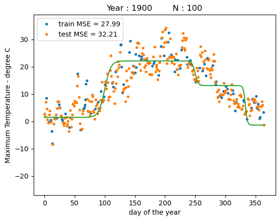
We see that we obtain the nearly identical solution to the version using gradient descent. However, in this version it would require some additional work to optimize over the basis function parameters.
Quadratic Optimization Problems#
Many problems in machine learning and statistics reduce to minimizing a quadratic function of the form
where \(\mathbf{A} \in \mathbb{R}^{d \times d}\) is a symmetric positive definite matrix, and \(\mathbf{b} \in \mathbb{R}^d\). The minimum of this function can be found analytically by setting the gradient to zero:
Ridge Regression as a Special Case#
The Ridge Regression objective can be rewritten in this general form. Starting from:
we expand the squared norm:
Dropping the constant term \(\frac{1}{2} \mathbf{y}^\top \mathbf{y}\), the expression becomes:
This matches the generalized quadratic form with:
\(\mathbf{A} = \mathbf{X}^\top \mathbf{X} + \lambda \mathbf{I}\)
\(\mathbf{b} = \mathbf{X}^\top \mathbf{y}\)
Since \(\mathbf{A}\) is symmetric and positive definite for \(\lambda > 0\), the minimum is achieved at:
This perspective makes it clear that Ridge Regression is simply a quadratic optimization problem with a symmetric positive definite matrix, and therefore has a unique analytical solution. This also connects to broader optimization theory and prepares us to explore other models — including Bayesian linear regression, kernel methods, and even Newton’s method — through the lens of solving linear systems.