The chain rule#
Most functions that we wish to optimize are not completely arbitrary functions, but rather are composed of simpler functions which we know how to handle. The chain rule gives us a way to calculate derivatives for a composite function in terms of the derivatives of the simpler functions that make it up.
The chain rule from single-variable calculus should be familiar:
Let \(f: \mathbb{R} \to \mathbb{R}\) and \(g: \mathbb{R} \to \mathbb{R}\) be differentiable functions. If \(f\) is differentiable at \(u_0 = g(x_0)\) and \(g\) is differentiable at \(x_0\), then the composition \(( f \circ g)(x) = f\bigl(g(x)\bigr)\) is differentiable at \(x_0\), and we have
where \(\circ\) denotes function composition. A proof of the single-variable chain rule is in the Appendix.
There is a natural generalization of this rule to multivariate functions.
Theorem (Multivariate Chain Rule)
Suppose \(f : \mathbb{R}^m \to \mathbb{R}^k\) and \(g : \mathbb{R}^n \to \mathbb{R}^m\).
Then \(f \circ g : \mathbb{R}^n \to \mathbb{R}^k\) and
Proof. Proof of the Multivariate Chain Rule.
Write \(g=(g_1,\dots,g_m)\) and \(f=(f_1,\dots,f_k)\). Then the composite \((f\circ g)_i(x)=f_i\bigl(g(x)\bigr)\).
Its partial derivative w.r.t. the \(j\)-th input coordinate \(x_j\) is, by the single-variable chain rule on each coordinate,
In matrix form this says
which is exactly the \((i,j)\) entry of the product \(\mathbf J_f(g(x))\,\mathbf J_g(x)\).
Hence
◻
In the special case \(k = 1\) we have the following corollary since \(\nabla f = \mathbf{J}_f^{\!\top\!}\).
Corollary (Chain Rule for Scalar-Valued Functions)
Suppose \(f : \mathbb{R}^m \to \mathbb{R}\) and \(g : \mathbb{R}^n \to \mathbb{R}^m\). Then \(f \circ g : \mathbb{R}^n \to \mathbb{R}\) and
Proof. Proof of the Scalar‐Valued Chain Rule.
When \(k=1\), \(f\colon\mathbb{R}^m\to\mathbb{R}\) has Jacobian \(\mathbf J_f(u)\) which is a \(1\times m\) row vector, and its gradient is \(\nabla f(u)=\mathbf J_f(u)^{\!\top}\). Applying the matrix‐chain result:
Thus
◻
Chain Rule for Basis Function Regression#
Now we can apply the chain rule to optimize the hyperparameters of the tanh basis functions in the context of our temperature prediction example. We still have to modify our ridge regression code to use the tanh basis function class and enable optimization over the hyperparameters using the chain rule.
So, let’s derive the Jacobian of ridge regression with respect to the hyperparameter matrix \(\mathbf{W}_\phi\) of the basis functions \(\mathbf{\phi}(\mathbf{x}): \mathbb{R}^D \to \mathbb{R}^K\).
Let’s have a look in how the basis functions affect the loss function.
Let \(f\) be the loss function, which is a function of the weights \(\mathbf{w}\) and the hyperparameters \(\mathbf{W}_\phi\) be the matrix of hyperparameters of the tanh basis functions. The loss function is given by:
where each of the \(l_n\) is the squared error for the prediction of the \(n\)-th data point and where we have added a quadratic regularizer on the entries of \(\mathbf{W}\).
When combining all \(N\) transformed input data points \(\boldsymbol{\phi(\mathbf{x}_n;\mathbf{W}_\phi)}\) into the transformed design matrix \(\boldsymbol{\Phi}(\mathbf{W}_\phi) \in\mathbb{R}^{N,P}\), and all the labels into the vector \(\mathbf{y}\in\mathbb{R}^N\), we get
Let \(\mathbf{J}_\phi\) be the Jacobian of the tanh basis functions with respect to the hyperparameters \(\mathbf{W}_\phi\), as we have derived in the last section.
As the loss is scalar, we can apply the Chain Rule for Scalar-Valued Functions.
Note that we have defined the non-zero part of \(\mathbf{J}_\Phi(\mathbf{W}_\phi)\) as a tensor of dimensionality \(N\)-by-\(D+1\)-by-\(K\).
So in our implementation we will have to be careful in how we carry out the multiplication, as we do not have implemented the remaining zero-dimensions.
The missing ingredient that we need to derive is \(\nabla_{\mathbf{W}_\phi} L(\mathbf{w}, \mathbf{W}_\phi)\). If we change \(\mathbf{W}_\phi\) we are changing the data representation that goes into the regression function. It follows that in contrast to the gradient that we used to optimize the ridge regression weights, we now have to take the gradient of the mean squared error with respect to the input data dimensions.
Let’s start by computing the gradient of the squared error \(l_n\) for the \(n\)-th data point only:
This gradient is a vector of length \(D+1\). It follows that the gradient for the loss \(L\) over the whole training data set, will be a vector of length \((D+1)N\), i.e. the concatenation of the \(N\) gradient vectors of all the \(l_N\). As for implementation purposes it is useful to keep track of the sample indices and the dimension indices, we write this gradient as the \(N\)-by-\((D+1)\) matrix \(\nabla_{\boldsymbol{\Phi}} L(\mathbf{w}, \mathbf{W}_\phi)\)
Alternatively, we could have used matrix derivatives to directly derive \(\nabla_{\boldsymbol{\Phi}} L(\mathbf{w}, \mathbf{W}_\phi)\) as
where \(\otimes\) is the outer product between the two vectors.
Let’s integrate this term into our ridge regression implementation:
import numpy as np

class BasisFunctionRidgeRegressionGD:
    def __init__(self, basis_function, learning_rate=0.01, num_iterations=1000, ridge=0.1, ridge_basis=0.1):
        self.basis_function = basis_function
        self.learning_rate = learning_rate
        self.num_iterations = num_iterations
        self.ridge = ridge
        self.ridge_basis = ridge_basis
        self.w = None

    def mse(self, X, y):
        # Mean Squared Error
        residuals = (y - self.pred(X))
        return np.mean(residuals*residuals)

    def d_loss_d_Phi(self, Phi, y):
        # gradient of the mean squared error w.r.t. Phi
        N = Phi.shape[0]
        if self.w is None:
            self.w = np.zeros(Phi.shape[1])
        residuals = (y - Phi @ self.w)
        return -residuals[:,np.newaxis] * self.w[np.newaxis,:] / N

    def loss(self, X, y):
        Phi = self.basis_function.transform(X)
        residuals = (y - Phi @ self.w)
        mse = np.mean(residuals*residuals)
        L = 0.5*mse + 0.5*self.ridge*np.sum(self.w**2)
        # add penalty on basis‐params:
        L += 0.5*self.ridge_basis*np.sum(self.basis_function.W**2)
        return L

    def gradient_w(self, X, y):
        # Gradient of the loss
        return -(self.basis_function.transform(X).T @ (y - self.pred(X))) / len(y) + self.ridge * self.w

    def gradient_basis_function(self, X, y):
        # Gradient of the loss
        return -self.w[np.newaxis,:] * (y - self.pred(X))[:,np.newaxis] / len(y)

    def gradient_basis_function_W(self, X, y):
        grad_loss_bf = self.gradient_basis_function(X, y)      # shape (N,P)
        jacobian_phi = self.basis_function.jacobian(X)     # shape (N,D+1,P)
        # chain‐rule: dL/dW_phi = sum_i grad_bf[i] • jacobian_phi[i]
        res = grad_loss_bf[:, None, :] * jacobian_phi          # (N, D+1, P)
        gW = res.sum(0)                                    # (D+1, P)
        # optional L2 on W:
        gW += self.ridge_basis * self.basis_function.W
        return gW

    def fit(self, X, y):
        Phi = self.basis_function.transform(X)
        # self.w = np.random.randn(Phi.shape[1])*0.001
        self.w = np.zeros(Phi.shape[1])
        for it in range(self.num_iterations):
            gW = self.gradient_basis_function_W(X, y)
            grad_w = self.gradient_w(X, y)
            # update basis function W and w
            self.basis_function.W -= self.learning_rate * gW
            self.w -= self.learning_rate * grad_w

    def pred(self, X):
        Phi = self.basis_function.transform(X)
        if self.w is None:
            self.w = np.zeros(Phi.shape[1])
        return Phi @ self.w

    def numerical_grad_W(self, X, y, eps=1e-7):
        """
        Numerically approximate dL/dW by central finite differences.
        Returns an array of the same shape as self.basis_function.W.
        """
        W = self.basis_function.W
        num_grad = np.zeros_like(W)
        # flatten indices
        it = np.nditer(W, flags=['multi_index'], op_flags=['readwrite'])
        while not it.finished:
            idx = it.multi_index
            orig = W[idx]
            # f(W + eps)
            W[idx] = orig + eps
            loss_plus = self.loss(X, y)
            # f(W - eps)
            W[idx] = orig - eps
            loss_minus = self.loss(X, y)
            # central difference
            num_grad[idx] = (loss_plus - loss_minus) / (2*eps)
            # restore
            W[idx] = orig
            it.iternext()
        return num_grad
Now, we have all the pieces together, to apply our new linear regression implementation to the temperature prediction problem, to fit the three tanh basis functions to the temperature data.
Show code cell source
import numpy as np
import pandas as pd
import matplotlib.pyplot as plt

class TanhBasis:
    def __init__(self, W):
        """
        W: array of shape (D+1, P), where
        - W[:D, k] are the slopes a_dk for each input dimension d and unit k
        - W[D, k] is the bias b_k for unit k.
        """
        self.W = W.copy()

    def Z(self, X):
        """Compute the product of the input data and the weights."""
        if len(X.shape) == 1:
            X = X[:, np.newaxis]
        return X @ self.W[:-1] + self.W[-1]

    def transform(self, X):
        """Compute the tanh basis functions."""
        return np.tanh(self.Z(X))

    def jacobian(self, X):
        """Compute the Jacobian of the tanh basis functions."""
        if len(X.shape) == 1:
            X = X[:, np.newaxis]
        dZ_dW = np.hstack((X, np.ones((X.shape[0], 1)))) # shape (N,D+1)
        dPhi_dz = (1 - np.tanh(self.Z(X))**2)   # shape (N,P)
        return dZ_dW[:,:,np.newaxis] * dPhi_dz[:,np.newaxis,:] # shape (N,D+1,P)

    def numerical_jacobian(self, X, eps=1e-6):
        """
        Numerically approximate the Jacobian of transform(X) wrt W.
        Returns an array of shape (n, d+1, p).
        """
        original_W = self.W.copy()
        N, D = X.shape
        K = self.W.shape[1]
        num_J = np.zeros((N, D+1, K))
        # iterate over each parameter j,k
        for d in range(D+1):
            for k in range(K):
                # perturb up
                self.W = original_W.copy()
                self.W[d, k] += eps
                phi_plus = self.transform(X)
                # perturb down
                self.W = original_W.copy()
                self.W[d, k] -= eps
                phi_minus = self.transform(X)
                # central difference
                num_J[:, d, k] = (phi_plus[:, k] - phi_minus[:, k]) / (2 * eps)
        # restore W
        self.W = original_W
        return num_J

YEAR = 1900
def load_weather_data(year = None):
    """
    load data from a weather station in Potsdam
    """

    names = ['station', 'date' , 'type', 'measurement', 'e1','e2', 'E', 'e3']
    data = pd.read_csv('../../datasets/weatherstations/GM000003342.csv', names = names, low_memory=False) # 47876 rows, 8 columns
    # convert the date column to datetime format
    data['date'] = pd.to_datetime(data['date'], format="%Y%m%d") # 47876 unique days
    types = data['type'].unique()

    tmax = data[data['type']=='TMAX'][['date','measurement']] # Maximum temperature (tenths of degrees C), 47876
    tmin = data[data['type']=='TMIN'][['date','measurement']] # Minimum temperature (tenths of degrees C), 47876
    prcp = data[data['type']=='PRCP'][['date','measurement']] # Precipitation (tenths of mm), 47876
    snwd = data[data['type']=='SNWD'][['date','measurement']] # Snow depth (mm), different shape
    tavg = data[data['type']=='TAVG'][['date','measurement']] # average temperature, different shape 1386
    arr = np.array([tmax.measurement.values,tmin.measurement.values, prcp.measurement.values]).T

    df = pd.DataFrame(arr/10.0, index=tmin.date, columns=['TMAX', 'TMIN', 'PRCP']) # compile data in a dataframe and convert temperatures to degrees C, precipitation to mm

    if year is not None:
        df = df[pd.to_datetime(f'{year}-1-1'):pd.to_datetime(f'{year}-12-31')]

    df['days'] = (df.index - df.index.min()).days
    return df

# Load weather data for the year 2000
df = load_weather_data(year = YEAR)

np.random.seed(2)
idx = np.random.permutation(df.shape[0])

idx_train = idx[0:100]
idx_test = idx[100:]

data_train = df.iloc[idx_train]
data_test = df.iloc[idx_test]

N_train = 100

a = np.array([.1, .2, .3])
b = np.array([-10.0,-50.0,-100.0])
W = np.array([a, b])

# tanh_basis = TanhBasis(W)
tanh_basis = TanhBasis(W)

ridge = 0.1     # strength of the L2 penalty in ridge regression
ridge_basis = 0.1     # strength of the L2 penalty on the parameters of the basis function

x_train = data_train.days.values[:N_train][:,np.newaxis] * 1.0
# X_train = tanh_basis(x_train, a, b)
y_train = data_train.TMAX.values[:N_train]

reg = BasisFunctionRidgeRegressionGD(basis_function=tanh_basis,ridge=ridge, learning_rate=0.00001, num_iterations=1000000, ridge_basis=ridge_basis)
reg.fit(x_train, y_train)

x_days = np.arange(366)[:,np.newaxis]
y_days_pred = reg.pred(x_days)

x_test = data_test.days.values[:,np.newaxis] * 1.0
y_test = data_test.TMAX.values
y_test_pred = reg.pred(x_test)
print("training MSE : %.4f" % reg.mse(x_train, y_train))
print("test MSE     : %.4f" % reg.mse(x_test, y_test))


fig = plt.figure()
ax = plt.plot(x_train,y_train,'.')
ax = plt.plot(x_test,y_test,'.')
ax = plt.legend(["train MSE = %.2f" % reg.mse(x_train, y_train),"test MSE = %.2f" % reg.mse(x_test, y_test)])
ax = plt.plot(x_days,y_days_pred)
ax = plt.ylim([-27,39])
ax = plt.xlabel("day of the year")
ax = plt.ylabel("Maximum Temperature - degree C")
ax = plt.title("Year : %i        N : %i" % (YEAR, N_train))
training MSE : 20.0247
test MSE     : 20.5147
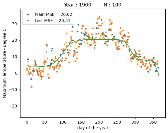
After fitting, we observe that the first sigmoid function has been stretched out to fit most of the first half year to model the increase in temperature up to summer and the second sigmoid basis function models the temperature decrease into the winter. The third basis function seems to overfit to some points at the end of the yet. Overall, both the train MSE and the test MSE have been drastically decreased compared to our hand-picked basis functions before.
Chain rule and the back-propagation algorithm#
Note that the model that we have derived represents a fully-connected neural network with a single hidden layer and the tanh activation function, or if we also count the output layer, this would be a 2-layer neural network. In the neural network world, the transformed data \(\boldsymbol\Phi(\mathbf{X}; \mathbf{W}_\phi)\) would correspond to the nodes on the hidden layer of the neural network and the parameter matrix \(\mathbf{W}_\phi\) would correspond to the weights of the hidden layer.
We have used the chain rule to compute the the gradient of \(L\) with respect to \(\mathbf{W}_\phi\). It turns out that neural networks use the back-propagation algorithm to compute such grtadients. The back-propagation is fundamentally based on the chain rule. However, it represents a more efficient implementation than the one that we have used here, as it would organize all copmutations into a forward pass that computes all the network layers up to the loss functions, while caching all the intermediate computations, and a backward pass, where it traces the network back towards the input and re-using all cached terms. Our implementation does not make use of caching and thus would be slower than the back-propagation algorithm.
Now, from a deep learning perspective, our 2-layer neural network would still be considered fairly shallow. If you would like to learn more about the back-propagation algorithm and how to build and train massively deep neural network architectures, check out the excellent Dive into Deep Learning online book.