First-order condition for local minima#
So far, we have used the gradient descent algorithm by taking a fixed number of small steps in the direction of the negative gradient. However, we have not yet established, when we can stop the algorithm.
Remember from single variable calculus that the first-order condition for a local minimum is that the derivative vanishes at that point.
The same is true in higher dimensions. The first-order condition for a local minimum of a function \(f : \mathbb{R}^n \to \mathbb{R}\) is that the gradient \(\nabla f(\mathbf{x})\) vanishes at that point.
Theorem (First-order condition)
Let \(f : \mathbb{R}^n \to \mathbb{R}\) be a function that is continuously differentiable in a neighborhood of \(\mathbf{x}^*\).
If \(\mathbf{x}^*\) is a local minimum of \(f\), then \(\nabla f(\mathbf{x}^*) = \mathbf{0}\).
This means that the gradient must vanish at any local minimum. Note that this is a necessary condition for a local minimum, but not a sufficient one. In other words, if \(\nabla f(\mathbf{x}^*) \neq \mathbf{0}\), then \(\mathbf{x}^*\) cannot be a local minimum. The converse is not true: there are points where the gradient vanishes which are not local minima.
Proof. Let \(\mathbf{x}^*\) be a local minimum of \(f\), and suppose towards a contradiction that \(\nabla f(\mathbf{x}^*) \neq \mathbf{0}\).
Let \(\mathbf{h} = -\nabla f(\mathbf{x}^*)\), noting that by the continuity of \(\nabla f\) we have
Hence
Thus there exists \(T > 0\) such that \(\mathbf{h}^{\!\top\!}\nabla f(\mathbf{x}^* + t\mathbf{h}) < 0\) for all \(t \in [0,T]\).
Let’s look at the line segment connecting \(\mathbf{x}^*\) and \(\mathbf{x}^* + t\mathbf{h}\).
From the Mean Value Theorem in Several Variables, we have that for any \(\mathbf{h} \in \mathbb{R}^n\) and \(t \in (0,T]\), there exists a point on that line segment parametrized by \(t' \in (0,t)\) such that
As we have chosen \(T\) small enough such that \(\mathbf{h}^{\!\top\!}\nabla f(\mathbf{x}^* + t'\mathbf{h}) < 0\), we have
whence it follows that \(\mathbf{x}^*\) is not a local minimum, a contradiction.
Hence \(\nabla f(\mathbf{x}^*) = \mathbf{0}\). ◻
The proof shows us why the vanishing gradient is necessary for an extremum: if \(\nabla f(\mathbf{x})\) is nonzero, there always exists a sufficiently small step \(\alpha > 0\) such that \(f(\mathbf{x} - \alpha\nabla f(\mathbf{x}))) < f(\mathbf{x})\). For this reason, \(-\nabla f(\mathbf{x})\) is called a descent direction.
So the gradient descent algorithm will take a step in the direction of the negative gradient until it reaches a stationary point where the gradient is zero. However, a zero gradient does not guarantee a minimum — only that the point is stationary.
✅ Example 1: A Local Minimum#
Let’s use the function:
Gradient:
\[\begin{split} \nabla f(x, y) = \begin{bmatrix} 2x \\ 2y \end{bmatrix}, \quad \Rightarrow \nabla f(0,0) = \begin{bmatrix} 0 \\ 0 \end{bmatrix}. \end{split}\]The origin \((0, 0)\) is a strict local minimum, since all directions lead upward: \(f(x, y) > f(0, 0) = 0\) for any \((x, y) \ne (0, 0)\).
❗ Example 2: A Saddle Point#
The function
also has a gradient of zero at the origin \((0, 0)\):
But it’s a saddle point:
It’s a minimum along the line \(y = 0\): \(f(x, 0) = x^2\).
It’s a maximum along the line \(x = 0\): \(f(0, y) = -y^2\).
So the gradient vanishes, but the point is not a local extremum.
Show code cell source
import numpy as np
import matplotlib.pyplot as plt
from mpl_toolkits.mplot3d import Axes3D

# Define the functions
def f_min(x, y):
    return x**2 + y**2

def f_saddle(x, y):
    return x**2 - y**2

# Create grid
x = np.linspace(-2, 2, 400)
y = np.linspace(-2, 2, 400)
X, Y = np.meshgrid(x, y)
Z_min = f_min(X, Y)
Z_saddle = f_saddle(X, Y)

# Plotting
fig = plt.figure(figsize=(14, 6))

# Plot for minimum
ax1 = fig.add_subplot(1, 2, 1, projection='3d')
ax1.plot_surface(X, Y, Z_min, cmap='viridis', alpha=0.9)
ax1.set_title('Local Minimum: $f(x, y) = x^2 + y^2$')
ax1.set_xlabel('x')
ax1.set_ylabel('y')
ax1.set_zlabel('f(x, y)')
ax1.scatter(0, 0, 0, color='red', s=50, label='Minimum at (0,0)')
ax1.legend()

# Plot for saddle
ax2 = fig.add_subplot(1, 2, 2, projection='3d')
ax2.plot_surface(X, Y, Z_saddle, cmap='coolwarm', alpha=0.9)
ax2.set_title('Saddle Point: $f(x, y) = x^2 - y^2$')
ax2.set_xlabel('x')
ax2.set_ylabel('y')
ax2.set_zlabel('f(x, y)')
ax2.scatter(0, 0, 0, color='black', s=50, label='Saddle at (0,0)')
ax2.legend()

plt.tight_layout()
plt.show()
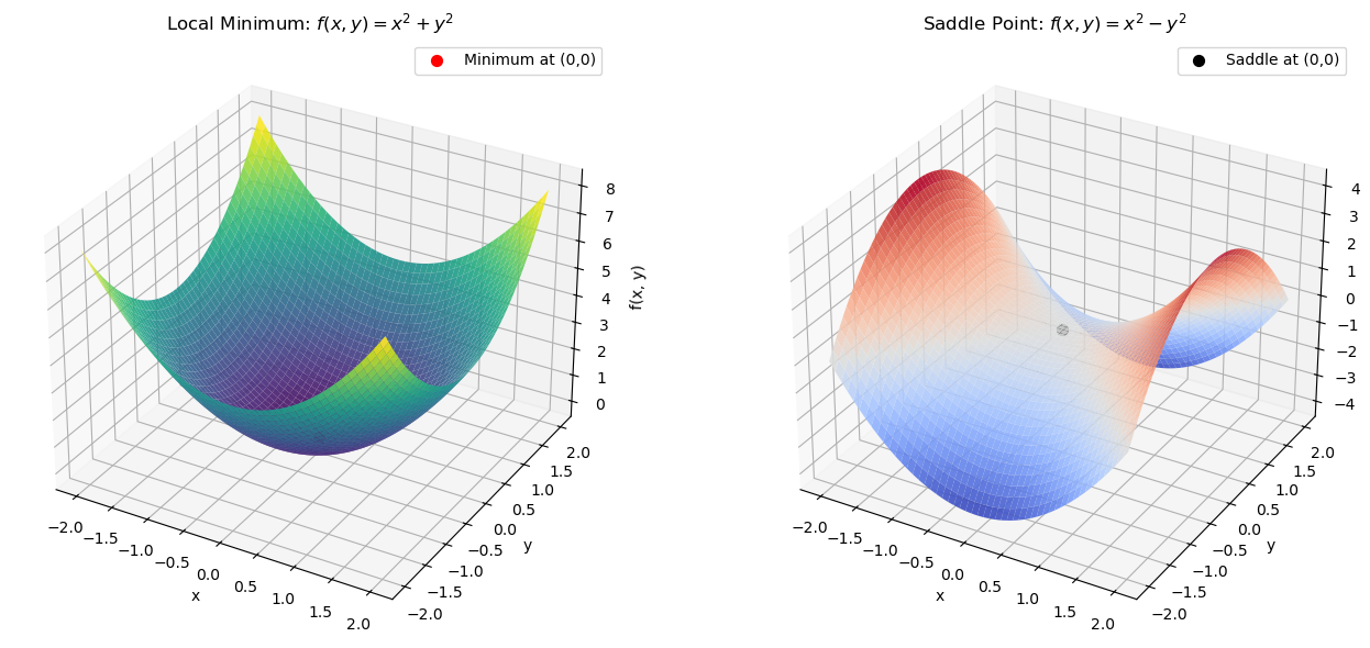
Left: \(f(x, y) = x^2 + y^2\) → Local minimum
The surface is a paraboloid opening upward.
Every direction from the origin increases the function value.
The gradient vanishes at the bottom: \(\nabla f(0,0) = 0\).
The Hessian is positive definite → confirms local minimum.
Right: \(f(x, y) = x^2 - y^2\) → Saddle point
A hyperbolic surface: increasing along \(x\), decreasing along \(y\).
Gradient vanishes at the origin, but there is no extremum.
This is the classic counterexample where the gradient condition is met, but the point is not a minimum or maximum.
🧠 Summary#
If a point is a local minimum, the gradient must be zero.
But a zero gradient alone is not enough — Over the next sections we will learn the second-order conditions based on the Hessian matrix, which tells us about the curvature of the function and will allow us to check if it’s a minimum, maximum, or saddle point.