The Squeeze Theorem

Theorem (Squeeze theorem)

Let \(g(x), h(x), f(x)\) be functions defined near \(c\). Suppose that there is an open interval around \(c\), except possibly at \(c\) itself, such that:

\[ g(x) \;\leq\; f(x) \;\leq\; h(x)\quad\text{for all } x\neq c. \]

If

\[ \lim_{x \to c} g(x) = \lim_{x \to c} h(x) = L, \]

then

\[ \lim_{x \to c} f(x) = L. \]

The squeeze theorem (also called the sandwich theorem) intuitively says that if a function \(f(x)\) is “trapped” or “squeezed” between two other functions \(g(x)\) and \(h(x)\) that both approach the same limit \(L\), then the squeezed function \(f(x)\) must also approach that same limit \(L\). This is particularly useful for evaluating limits of complicated functions by bounding them with simpler ones whose limits we already know.

---

Proof. Squeeze theorem.

Step 1: Set up the assumptions clearly. We have three functions \(g(x), f(x), h(x)\) satisfying:

\[ g(x) \leq f(x) \leq h(x),\quad \text{for all } x \text{ near } c, x \neq c, \]

and we have the limit conditions:

\[ \lim_{x\to c} g(x) = L \quad \text{and} \quad \lim_{x\to c} h(x) = L. \]

Let’s prove that \(\lim_{x\to c} f(x) = L\).

Step 2: Use the definition of limit. By definition of limits, for any \(\varepsilon > 0\), there exists some \(\delta > 0\) such that whenever \(0 < |x - c| < \delta\):

• For \(g(x)\):

\[ |g(x)-L| < \varepsilon \quad\Longleftrightarrow\quad L-\varepsilon < g(x) < L+\varepsilon. \]

• For \(h(x)\):

\[ |h(x)-L| < \varepsilon \quad\Longleftrightarrow\quad L-\varepsilon < h(x) < L+\varepsilon. \]

Step 3: Combine inequalities. From these two inequalities, for \(0 < |x-c|<\delta\), we have:

• Lower bound:

  \[ g(x) > L-\varepsilon. \]

• Upper bound:

  \[ h(x) < L+\varepsilon. \]

Thus, combining these with the given inequalities for \(f(x)\):

\[ L-\varepsilon \;<\; g(x) \;\leq\; f(x) \;\leq\; h(x) \;<\; L+\varepsilon. \]

Hence, for any \(\varepsilon >0\), there exists a \(\delta > 0\), such that if \(0 < |x-c| < \delta\):

\[ |f(x)-L|<\varepsilon. \]

This precisely matches the definition of the limit \(\lim_{x\to c} f(x)=L\).

Step 4: Conclusion. Thus, by definition of the limit, we have:

\[ \lim_{x\to c} f(x)=L, \]

which proves the squeeze theorem. ◻

Here’s the visualization of a function \(f(x)\), which oscillates between a lower bound \(g(x)\) and an upper bound \(h(x)\).

The bounding functions \(g(x)\) and \(h(x)\) are defined as:

\[ g(x) = x^2 \cos\left(\frac{1}{x}\right) - x^2 \quad \text{ and } \quad h(x) = x^2 \cos\left(\frac{1}{x}\right) + x^2 \]

As \(x\) approaches the limit point \(c=0\), both \(g(x)\) and \(h(x)\) approach \(0\), squeezing the function \(f(x)\) to also approach \(0\).

Show code cell source Hide code cell source

import numpy as np
import matplotlib.pyplot as plt

# Define the functions
def g(x):
    return x**2 * np.cos(1/x) - x**2

def h(x):
    return x**2 * np.cos(1/x) + x**2

def f(x):
    return x**2 * np.cos(1/x)

# Define the x values (avoiding division by zero)
x = np.linspace(-0.1, 0.1, 1000)
x = x[x != 0]

# Plot the functions
plt.figure(figsize=(10,6))
plt.plot(x, g(x), label='$g(x)$ (lower bound)', color='green', linestyle='--')
plt.plot(x, h(x), label='$h(x)$ (upper bound)', color='blue', linestyle='--')
plt.plot(x, f(x), label='$f(x)$ (squeezed)', color='red')

# Limit point c=0
plt.scatter(0, 0, color='black', zorder=5, label='Limit at $c=0$')

# Formatting the plot
plt.title('Visualization of the Squeeze Theorem')
plt.xlabel('$x$')
plt.ylabel('Function values')
plt.axhline(0, color='black', lw=0.5)
plt.axvline(0, color='black', lw=0.5)
plt.legend()
plt.grid(True)
plt.show()

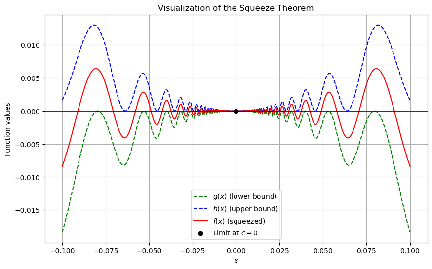
The red function \(f(x)\) is “squeezed” between the green \(g(x)\) and blue \(h(x)\) functions as \(x \to 0\). Both the upper and lower bounding functions approach zero, forcing the squeezed function \(f(x)\) to approach zero as well.