The Jacobian

The Jacobian#

In machine learning, most of the time we’re optimizing a scalar “loss,” but internally the models we train are often vector-valued mappings.

Wherever you see a function with multiple outputs, like

\[ f: \mathbb{R}^n \;\longrightarrow\; \mathbb{R}^m \]

you’ll want its Jacobian.

The Jacobian is the matrix of first-order partial derivatives of each output of \(f\) with respect to each of the input dimensions. It generalizes the gradient of a scalar-valued function to vector-valued functions.

\[\begin{split}\mathbf{J}_f = \begin{bmatrix} \frac{\partial f_1}{\partial x_1} & \dots & \frac{\partial f_1}{\partial x_n} \\ \vdots & \ddots & \vdots \\ \frac{\partial f_m}{\partial x_1} & \dots & \frac{\partial f_m}{\partial x_n}\end{bmatrix} \hspace{0.5cm}\text{i.e.}\hspace{0.5cm} [\mathbf{J}_f]_{ij} = \frac{\partial f_i}{\partial x_j}\end{split}\]

Note the special case \(m = 1\), where \(\nabla f = \mathbf{J}_f^{\!\top\!}\).

Basis Functions and their Jacobians#

We have seen vector-valued functions in the context of basis functions such as the tanh basis functions that we used in the prediction of temperature as a function of the day in the year.

In the context of basis functions, we have a function \(\boldsymbol{\phi}\) that transforms the input data \(\mathbf{x}\) into a new feature space. The basis functions are typically parameterized by weights and biases, and they can be thought of as nonlinear transformations of the input data. The goal of using basis functions is to create a new feature space that can better capture the underlying structure of the data, allowing for more flexible modeling.

In order to optimize over the basis functions, we need to compute their Jacobian. What are the inputs and what are the outputs of the basis functions?

If we have \(K\) basis functions, these transform a \(D\)-dimensional feature vector \(\mathbf{x}\) into a \(K\)-dimensional vector \(\boldsymbol{\phi}_\boldsymbol{\theta}(\mathbf{x})\).

\[ \boldsymbol{\phi}_\boldsymbol{\theta}(\mathbf{x}): \mathbb{R}^D \rightarrow \mathbb{R}^K \]

Here, \(\boldsymbol{\theta}\) is the vector of parameters of \(\boldsymbol{\phi}\).

In machine learning our goal will be to optimize over these features based on a loss function computed over a fixed training data set of size \(N\) that is transformed using \(\boldsymbol{\phi}\). Thus, we need to understand how the transformed data features of the training data set change as we modify the parameters \(\boldsymbol{\theta}\).

In this view, we have to treat the parameters \(\boldsymbol{\theta}\) as the input and the transformed data set as the output of \(\boldsymbol{\phi}\).

\[ \boldsymbol{\phi}_{\mathbf{X}}(\boldsymbol{\theta}): \mathbb{R}^{P}\rightarrow\mathbb{R} ^{NK},\]

where \(P\) is the total number of parameters of all the basis functions.

Thus, the Jacobian will be a matrix of size \(P\) times \((NK)\).

To better keep track of the dimensions, we can think of the Jacobian as a \(P\)-by-\(K\) matrix for each data point \(n\).

\[\begin{split} \mathbf{J}_{\boldsymbol{\phi}}(\mathbf{x}_n) = \begin{bmatrix} \frac{\partial \phi_{n1}}{\partial \theta_1} & \dots & \frac{\partial \phi_{n1}}{\partial \theta_P} \\ \vdots & \ddots & \vdots \\ \frac{\partial \phi_{nK}}{\partial \theta_1} & \dots & \frac{\partial \phi_{nK}}{\partial \theta_P}\end{bmatrix} \hspace{0.5cm}\text{i.e.}\hspace{0.5cm} [\mathbf{J}_{\boldsymbol{\phi}}]_{n, k; p} = \frac{\partial \phi_{nk}}{\partial \theta_p} \end{split}\]

where \(n\) is the index of the data point, \(k\) is the index of the basis function, and \(p\) is the index of the parameter.

Jacobian of tanh basis functions#

Let’s apply this to an example, where we transform the data using \(K\) tanh basis functions.

Let \(\phi_{nk}\) be the \(k\)-th basis-function activation on the \(n\)-th sample.

\[ \phi_{nk} =\tanh\!\bigl(z_{nk}\bigr) \quad\text{with}\quad z_{nk} \;=\;\sum_{d=1}^D a_{dk}\,x_{nd}\;+\;b_k \]

So, the parameters of the basis functions are the weights \(a_{dk}\) and the biases \(b_k\). The weights \(a_{dk}\) are the slopes of the \(k\)-th basis function with respect to the \(d\)-th input feature, and the biases \(b_k\) are the offsets of the \(k\)-th basis function.

Partial derivative for the weights \(a_{kd}\)#

\[ \frac{\partial\,\phi_{nk}}{\partial\,a_{d\ell}} \quad,\quad d\in\{1,\dots,D\},\;k,\ell\in\{1,\dots,K\}. \]

1. Chain-rule decomposition#

By the chain rule,

\[ \frac{\partial\,\phi_{nk}}{\partial\,a_{d\ell}} =\underbrace{\frac{d}{dz}\tanh(z)\Big|_{z=z_{nk}}}_{\tanh'(z_{nk})} \;\times\; \frac{\partial\,z_{nk}}{\partial\,a_{d\ell}}. \]

2. Compute each factor#

Derivative of tanh

\[ \frac{d}{dz}\tanh(z) =1 - \tanh^2(z) \;\;\;\Longrightarrow\;\;\; \tanh'(z_{nk}) = 1 - \tanh^2\bigl(z_{nk}\bigr) = 1 - \phi_{nk}^2. \]
Derivative of the affine argument

\[\begin{split} z_{nk} = \sum_{d=1}^D a_{dk}\,x_{nd} + b_k \quad\Longrightarrow\quad \frac{\partial z_{nk}}{\partial a_{d\ell}} = \begin{cases} x_{nd}, & \ell = k,\\ 0, & \ell \neq k. \end{cases} \end{split}\]

3. Put it together#

Hence

\[\begin{split} \boxed{ \frac{\partial\,\phi_{nk}}{\partial\,a_{d\ell}} = \begin{cases} \bigl(1 - \phi_{nk}^2\bigr)\;x_{nd}, & \ell=k,\\ 0, & \ell\neq k. \end{cases} } \end{split}\]

Equivalently, in one expression using the Kronecker delta \(\delta_{\ell k}\):

\[ \frac{\partial\,\phi_{nk}}{\partial\,a_{d\ell}} = \delta_{\ell k}\;\bigl(1 - \phi_{nk}^2\bigr)\;x_{nd}. \]

We can see that the Jacobian has plenty of zeros, as the parameter of the \(k\)-th basis function only have an effect on the output of the \(k\)-th basis function and thus the partial derivatives for all the other basis functions are zero. This is a consequence of the fact that the tanh basis functions are independent of each other.

Matrix-form view#

If we collect all \(\phi_{nk}\) into an \(N\times K\) matrix \(\boldsymbol{\Phi}\), and all weights \(a_{dk}\) into a \(D\times K\) matrix \(\mathbf{A}\), then the Jacobian \(\tfrac{\partial\,\boldsymbol{\Phi}}{\partial\,\mathbf{A}}\) is a 4-tensor with entries

\[ \bigl[J_{\boldsymbol{\Phi},\mathbf{A}}\bigr]_{\,n,k\,;\,d,\ell} =\frac{\partial\,\phi_{nk}}{\partial\,a_{d\ell}} =\delta_{\ell k}\,(1-\phi_{nk}^2)\,x_{nd}. \]

This observation allows us to simplify the implementation, as in practice, we only need to keep track of the non-zero part of the Jacobian.

For each basis unit \(k\) you get the non-zero gradient

\[ \nabla_{a_{\cdot k}}\phi_{\cdot k} =\bigl(1-\phi_{\cdot k}^2\bigr)\odot x_{\cdot\,:\,} \]

(where “\(\odot\)” is element-wise multiplication of the vector \(1-\phi_{nk}^2\) with each column of the design matrix).

Partial derivative for the weights \(b_k\)#

The non-zero part of the Jacobian with respect to the bias \(b_k\) is a vector of size \(N\) (one for each data point) and is given by:

\[ \frac{\partial\,\phi_{nk}}{\partial\,b_k} =\frac{d}{dz}\tanh(z)\Big|_{z=z_{nk}} =\frac{d}{dz}\tanh(z_{nk}) =1 - \tanh^2(z_{nk}) =1 - \phi_{nk}^2. \]

This shows how the tanh function responds to changes in the bias hyperparameter \(b_k\).

Let’s implement the tanh basis with a function jacobian(X) that returns the Jacobian matrix.

The returned Jacobian J has shape \((N,\,D+1,\,k)\) with

\[\begin{split} J[n,d,k] \;=\; \frac{\partial\,\phi_{n,k}}{\partial\,W_{d,k}} \;=\; \begin{cases} (1-\phi_{n,k}^2)\,X_{n,d}, & d<D\quad(\text{zero-based indexing}),\\ (1-\phi_{n,k}^2), & d=D\quad(\text{bias term}). \end{cases} \end{split}\]

Analytic derivations and implementations of Jacobians are always invovled and there are many ways to make errors. To assert that the implementation is correct, we added a numerical_jacobian(X, eps) method to the TanhBasis class. It perturbs each parameter \(W_{d,k}\) by \(\pm\varepsilon\), recomputes the activations, and uses a central difference to numerically approximate

\[ \frac{\partial \phi_{n,k}}{\partial W_{d,k}} \equiv \frac{\phi_{n,k}(W_{d,k}+\varepsilon)\;-\;\phi_{n,k}(W_{d,k}-\varepsilon)}{2\varepsilon}. \]

import numpy as np

class TanhBasis:
    def __init__(self, W):
        """
        W: array of shape (D+1, P), where
        - W[:D, k] are the slopes a_dk for each input dimension d and unit k
        - W[D, k] is the bias b_k for unit k.
        """
        self.W = W.copy()

    def Z(self, X):
        """Compute the product of the input data and the weights."""
        if len(X.shape) == 1:
            X = X[:, np.newaxis]
        return X @ self.W[:-1] + self.W[-1]

    def transform(self, X):
        """Compute the tanh basis functions."""
        return np.tanh(self.Z(X))

    def jacobian(self, X):
        """Compute the Jacobian of the tanh basis functions."""
        if len(X.shape) == 1:
            X = X[:, np.newaxis]
        dZ_dW = np.hstack((X, np.ones((X.shape[0], 1)))) # shape (N,D+1)
        dPhi_dz = (1 - np.tanh(self.Z(X))**2)   # shape (N,P)
        return dZ_dW[:,:,np.newaxis] * dPhi_dz[:,np.newaxis,:] # shape (N,D+1,P)

    def numerical_jacobian(self, X, eps=1e-6):
        """
        Numerically approximate the Jacobian of transform(X) wrt W.
        Returns an array of shape (n, d+1, p).
        """
        original_W = self.W.copy()
        N, D = X.shape
        K = self.W.shape[1]
        num_J = np.zeros((N, D+1, K))
        # iterate over each parameter j,k
        for d in range(D+1):
            for k in range(K):
                # perturb up
                self.W = original_W.copy()
                self.W[d, k] += eps
                phi_plus = self.transform(X)
                # perturb down
                self.W = original_W.copy()
                self.W[d, k] -= eps
                phi_minus = self.transform(X)
                # central difference
                num_J[:, d, k] = (phi_plus[:, k] - phi_minus[:, k]) / (2 * eps)
        # restore W
        self.W = original_W
        return num_J

A quick comparison on random data shows the max absolute difference between analytic and numeric Jacobians is on the order of \(10^{-11}\), confirming that the analytic Jacobian is correctly implemented:

Max abs diff: 3.4030778195415223e-11

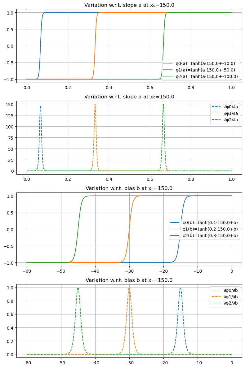
Visualizing the Jacobian of Tanh Basis Functions#

In the following, we visualize the three tanh basis functions that we used in the previous Section for temperature prediction and their Jacobians with respect to the slope \(a\), and bias \(b\). We will plot the three tanh basis functions and their Jacobians with respect to the slope \(a\), and bias \(b\).

∂φ/∂a (Jacobian w.r.t. the slope hyperparameter \(a\)) at a fixed 1-dimensional \(x_0\)
∂φ/∂b (Jacobian w.r.t. the bias hyperparameter \(b\)) at the same fixed 1-dimensional \(x_0\)

../_images/5ce05e09527ad988583cf67571ba5eb44939f3bba42e660641b5f807da5fc731.png

Before we can use the TanhBasis class with Jacobian to optimize over the hyperparameters in our ridge regression, we need to understand, how the Jacobian is used in the optimization process. The missing ingredient is the chain rule that we will discuss next.