Taylor’s Theorem#
Polynomials provide a framework for function approximation. It turns out, that many functions can be approximated well by so-called Taylor polynomials and that for a large class of infintely differentiable functions this approximation can be exact. We call this class of functions analytic.
We state and prove the first order Taylor’s Theorem with remainder in the multivariable case and state it in the second order, as is typically encountered in machine learning and optimization contexts.
We’ll first state the single-variable version, then the multivariable version (more relevant to gradient and Hessian-based methods), and give a proof for the single-variable case using the mean value form of the remainder.
Theorem (Taylor’s Theorem with Remainder (Single Variable))
Let \(f : \mathbb{R} \to \mathbb{R}\) be \((n+1)\)-times continuously differentiable on an open interval containing \(a\) and \(x\).
Then:
Where the remainder term is given by the Lagrange form:
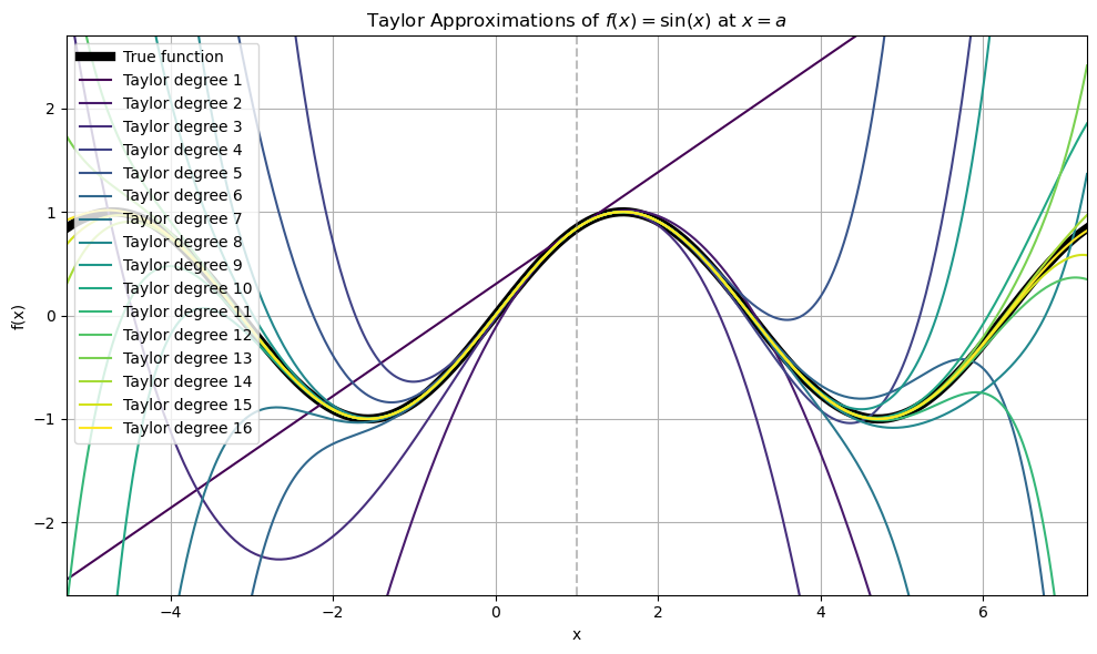
Let’s visualize a function \(f : \mathbb{R} \to \mathbb{R}\) along with its Taylor approximations of increasing degree \(n = 1, 2, \dots, N\) centered at a point \(a\). We overlay each approximation on the graph of the true function to show how the Taylor series converges.
Show code cell source
import numpy as np
import matplotlib.pyplot as plt
from math import factorial
import sympy as sp

# Define the function f symbolically
x = sp.symbols('x')
f_expr = sp.sin(x)  # Change this to any (n+1)-times differentiable function
f = sp.lambdify(x, f_expr, modules='numpy')

# Taylor expansion at point a
a = 1
N = 16  # Highest degree of Taylor polynomial to visualize
x_vals = np.linspace(-2*np.pi+a, 2*np.pi+a, 400)

# Generate the Taylor polynomial of degree n
def taylor_poly(expr, a, n):
    return sum((expr.diff(x, k).subs(x, a) / factorial(k)) * (x - a)**k for k in range(n+1))

# Plotting
fig, ax = plt.subplots(figsize=(10, 6))
plt.plot(x_vals, f(x_vals), label='True function', color='black', linewidth=6)

colors = plt.cm.viridis(np.linspace(0, 1, N))
for n in range(1, N+1):
    taylor_expr = taylor_poly(f_expr, a, n)
    taylor_func = sp.lambdify(x, taylor_expr, modules='numpy')
    plt.plot(x_vals, taylor_func(x_vals), label=f'Taylor degree {n}', color=colors[n-1])

plt.axvline(a, color='gray', linestyle='--', alpha=0.5)
plt.title(r'Taylor Approximations of $f(x) = \sin(x)$ at $x = {a}$')
plt.xlabel('x')
plt.ylabel('f(x)')
plt.legend()
plt.grid(True)
ax.set_ylim([-2.7,2.7])
ax.set_xlim([-2*np.pi+a, 2*np.pi+a])
plt.tight_layout()
plt.show()
Big-O Form of Taylor’s Remainder (Single Variable)#
Corollary
Let \(f: \mathbb{R} \to \mathbb{R}\) be \((n+1)\)-times continuously differentiable in a neighborhood of \(a\).
Then:
This means:
There exists a constant \(C\) and a neighborhood around \(a\) such that
\[ |R_{n+1}(x)| \leq C |x - a|^{n+1} \quad \text{as } x \to a \]
The notation tells us that the remainder vanishes at the same rate as \((x - a)^{n+1}\) as \(x \to a\).
Let’s prove Taylor’s Theorem with the exact expression for the remainder.
Proof. (Single Variable, Lagrange Form of the Remainder)
We want to prove that:
Step 1: Define the Taylor Polynomial and Remainder
Let
We want to find an expression for \(R_{n+1}(x)\).
Step 2: Define an Auxiliary Function
Define a function \(\phi(t)\) that measures the difference between \(f(t)\) and the Taylor polynomial + an extra term we choose to vanish at \(t = x\):
We designed this function such that:
\(\phi(a) = f(a) - T_n(a) - 0 = 0\) (since \(T_n(a) = f(a)\))
\(\phi(x) = f(x) - T_n(x) - \frac{f^{(n+1)}(x)}{(n+1)!}(x - a)^{n+1}\)
So \(\phi(x) = R_{n+1}(x) - \frac{f^{(n+1)}(x)}{(n+1)!}(x - a)^{n+1}\)
Now, the goal is to compare this to a function that we can analyze using Cauchy’s Mean Value Theorem.
Step 3: Construct a Function with a Known Root
Let:
and define:
Both \(F(t)\) and \(G(t)\) are \(C^1\) functions, and they vanish at \(t = a\): \(F(a) = G(a) = 0\)
We now apply Cauchy’s Mean Value Theorem to \(F\) and \(G\) on the interval \([a, x]\):
If \(F\) and \(G\) are differentiable and \(G'(t) \neq 0\) on \((a, x)\), then there exists \(\xi \in (a, x)\) such that:
\[\frac{F(x) - F(a)}{G(x) - G(a)} = \frac{F'(\xi)}{G'(\xi)}\]
Apply it:
\(F(x) - F(a) = \phi(x) - 0 = R_{n+1}(x) - \frac{f^{(n+1)}(x)}{(n+1)!}(x-a)^{n+1}\)
\(G(x) - G(a) = (x-a)^{n+1} - 0\)
So:
Compute \(\phi'(t)\):
\(\phi'(t) = f'(t) - T_n'(t) - \frac{f^{(n+1)}(x)}{(n+1)!} \cdot (n+1)(t - a)^n\)
But recall that \(T_n'(t) = \sum_{k=1}^n \frac{f^{(k)}(a)}{(k-1)!}(t - a)^{k-1}\), so \(\phi'(t)\) behaves like a difference between \(f'(t)\) and the Taylor expansion of \(f'\).
But instead of continuing with \(\phi(t)\), there’s a simpler and cleaner proof using a function designed for Lagrange’s form.
Using Cauchy’s Mean Value Theorem
Let’s define:
Note:
\(h(a) = 0\), because \(T_n(a) = f(a)\)
\(g(a) = 0\)
Then apply Cauchy’s Mean Value Theorem to \(h\) and \(g\) on \([a, x]\):
There exists \(\xi \in (a, x)\) such that:
Let’s compute:
\(g(x) = (x - a)^{n+1}\), and \(g'(\xi) = (n+1)(\xi - a)^n\)
\(h(x) = f(x) - T_n(x) = R_{n+1}(x)\)
\(h'(\xi) = f^{(n+1)}(\xi) \cdot \frac{(\xi - a)^n}{n!}\) (this is a known identity)
Then:
Q.E.D.
Analytic Functions#
Analytic functions are intimately related to Taylor series and to the remainder behavior.
🔍 What Is an Analytic Function?#
A function \(f : \mathbb{R} \to \mathbb{R}\) (or \(f : \mathbb{R}^d \to \mathbb{R}\)) is called analytic at a point \(a\) if:
The Taylor series of \(f\) at \(a\) converges to the function in a neighborhood of \(a\):
\[f(x) = \sum_{k=0}^{\infty} \frac{f^{(k)}(a)}{k!}(x - a)^k\quad \text{for all } x \text{ near } a\]
That is:
Not only does the Taylor series exist (i.e., \(f\) is infinitely differentiable),
But it converges to the true function (i.e., the remainder \(R_n(x) \to 0\) as \(n \to \infty\)).
🚫 Not All Smooth Functions Are Analytic#
An important subtlety:
There exist functions that are infinitely differentiable (smooth), but not analytic.
For example, the function
is \(C^\infty\) everywhere, but its Taylor series at 0 is identically zero (all derivatives vanish at 0) — even though the function is not identically zero.
Show code cell source
import numpy as np
import matplotlib.pyplot as plt
from math import factorial

# Define the smooth but non-analytic function
def f(x):
    out = np.zeros_like(x)
    nonzero = x != 0
    out[nonzero] = np.exp(-1 / x[nonzero]**2)
    return out

# Compute Taylor polynomials at x=0 (they are all zero)
def taylor_approx(x, n):
    return np.zeros_like(x)  # All derivatives at 0 are zero

# Set up x-values
x_vals = np.linspace(-1, 1, 400)
f_vals = f(x_vals)

# Plot the true function and several Taylor approximations
# Create the plot
fig, ax = plt.subplots(figsize=(10, 6))
ax.plot(x_vals, f_vals, label='$f(x) = e^{-1/x^2}$ (extended by 0 at 0)', color='black')

colors = plt.cm.viridis(np.linspace(0, 1, 5))
for n, c in zip([1, 3, 5, 10, 20], colors):
    plt.plot(x_vals, taylor_approx(x_vals, n), linestyle='--', color=c, label=f'Taylor degree {n}')

plt.axvline(0, color='gray', linestyle='--', alpha=0.5)
plt.title('Smooth but Non-Analytic Function at $x = 0$')
plt.xlabel('x')
plt.ylabel('f(x)')
ax.set_ylim([-0.03, 0.2])
ax.set_xlim([-0.75, 0.75])
plt.legend()
plt.grid(True)
plt.tight_layout()
plt.show()
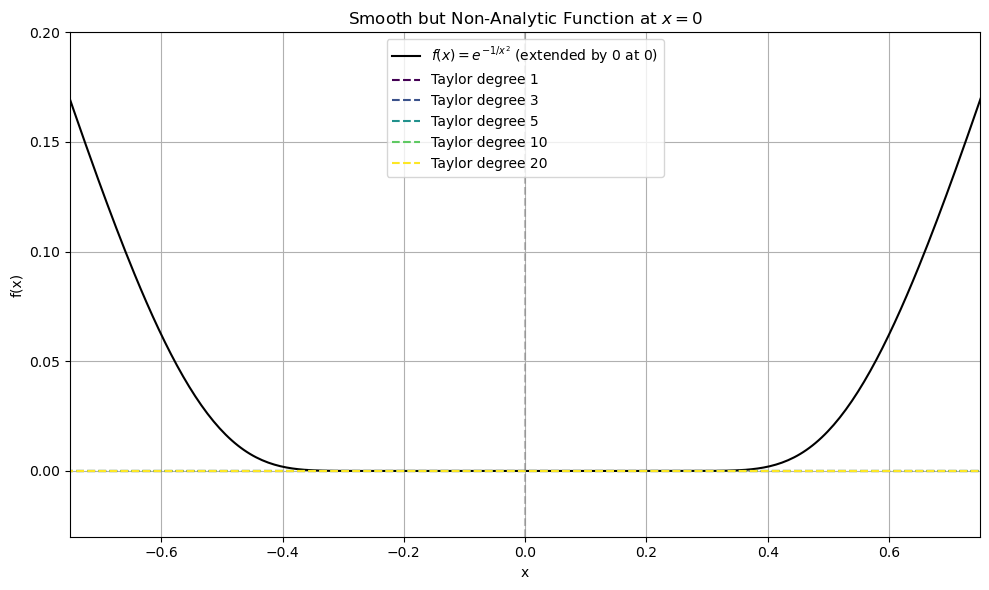
This function is infinitely differentiable (smooth) at \(x = 0\), but not analytic there: all of its derivatives at 0 vanish, so every Taylor polynomial is the zero function. Yet the function is clearly nonzero for any \(x \neq 0\).
The true function \(f(x)\) (black curve), sharply rising near zero.
All Taylor polynomials (dashed lines) are identically zero and fail to approximate the function anywhere except exactly at \(x = 0\).
So: ✅ smooth ≠ analytic ✅ analytic ⇒ smooth ❌ smooth ⇒ analytic
🔄 How This Relates to the Big-O Remainder#
The Big‑O bound tells you that the remainder goes to zero like \((x - a)^{n+1}\) near \(a\), for fixed \(n\).
But to be analytic, you need:
\[ \lim_{n \to \infty} R_n(x) = 0 \quad \text{for all } x \text{ in a neighborhood of } a \]i.e., convergence of the full infinite series, not just the rate of vanishing of each finite approximation.
So, Big-O bounds are necessary (they control approximation error), but not sufficient for analyticity. You need the entire remainder sequence \(R_n(x) \to 0\) for analytic behavior.
🧠 Summary Table#
Property |
What It Implies |
|---|---|
Smooth \(C^\infty\) |
All derivatives exist and are continuous |
Analytic |
Taylor series converges to function locally |
Big-O remainder |
Controls approximation error for fixed \(n\) |
\(R_n(x) \to 0\) |
Required for analyticity |
Taylor Expansion in Multiple Variables#
Recall, that we can create a locally linear approximation to a function at a point \(\mathbf{x}_0 \in \mathbb{R}^d \) using the gradient at \(\nabla f(\mathbf{x}_0)\).
This affine approximation is also known as the first-order Taylor approximation. It agrees with the original function in value and gradient at the point \( \mathbf{x}_0 \).
If you explicitly include the second-order term evaluated at \(\mathbf{x}_0\), then you’re writing the second-order Taylor expansion:
This is a local quadratic approximation to the function. It agrees with the original function in value, gradient, and Hessian at the point \( \mathbf{x}_0 \). The Hessian appears naturally in the second-order Taylor approximation of a function around a point \( \mathbf{x}_0 \in \mathbb{R}^d \).
The gradient term captures the linear behavior (slope) of the function near \( \mathbf{x}_0 \).
The Hessian term captures the curvature — how the gradient changes in different directions.
In this case, the remainder (if stated) would involve third derivatives, and the approximation is called second-order because you’re explicitly using second-order information in the main approximation.
We illustrate both the first-order and the second-order Taylor expansion using the following function.
We compute the first-order and second-order Taylor approximations at the point \( (x_0, y_0) = (0.3, 0.3) \).
The true function and the linear approximation match in value and gradient at the point \( (x_0, y_0)\) but differ elsewhere. Similarly, the quadratic approximation match in value, gradient, and Hessian at this point but differ elsewhere.
Show code cell source
import numpy as np
import matplotlib.pyplot as plt
from mpl_toolkits.mplot3d import Axes3D

# Define the function and its gradient and Hessian
f = lambda x, y: np.log(1 + x**2 + y**2)
x0, y0 = 0.3, 0.3

# Compute value, gradient, and Hessian at (x0, y0)
r2 = x0**2 + y0**2
f0 = np.log(1 + r2)
grad = np.array([2*x0, 2*y0]) / (1 + r2)
H = (2 / (1 + r2)) * np.eye(2) - (4 * np.outer([x0, y0], [x0, y0])) / (1 + r2)**2

# Taylor expansion up to second order
def f_taylor_first_order(x, y):
    dx = x - x0
    dy = y - y0
    delta = np.array([dx, dy])
    return f0 + (grad @ delta).sum()

# Taylor expansion up to second order
def f_taylor_second_order(x, y):
    dx = x - x0
    dy = y - y0
    delta = np.array([dx, dy])
    return f0 + (grad @ delta).sum() + 0.5 * (delta @ H @ delta).sum()

# Create grid for plotting
x_vals = np.linspace(x0-1, x0+1, 100)
y_vals = np.linspace(y0-1, y0+1, 100)
X, Y = np.meshgrid(x_vals, y_vals)
Z_true = f(X,Y)
Z_first = np.zeros(X.shape)
Z_second = np.zeros(X.shape)

for i in range(X.shape[0]):
    for j in range(X.shape[1]):
        Z_first[i,j] = f_taylor_first_order(X[i,j],Y[i,j])
        Z_second[i,j] = f_taylor_second_order(X[i,j],Y[i,j])

# Plot both Taylor approximations
fig = plt.figure(figsize=(14, 6))
ax1 = fig.add_subplot(1, 2, 1, projection='3d')
ax2 = fig.add_subplot(1, 2, 2, projection='3d')

true_surface1 = ax1.plot_surface(X, Y, Z_true, cmap='viridis', alpha=0.6)
approx_surface1 = ax1.plot_surface(X, Y, Z_first, cmap='coolwarm', alpha=0.7)
ax1.scatter(x0, y0, f0, color='red', s=50, label=r'$\mathbf{x}_0$')
ax1.set_title("First-Order Taylor Approximation")
ax1.set_xlabel("x")
ax1.set_ylabel("y")
ax1.legend()
ax1.set_zlim([-0.5,2])

true_surface2 = ax2.plot_surface(X, Y, Z_true, cmap='viridis', alpha=0.6)
approx_surface2 = ax2.plot_surface(X, Y, Z_second, cmap='coolwarm', alpha=0.7)
ax2.scatter(x0, y0, f0, color='red', s=50, label=r'$\mathbf{x}_0$')
ax2.set_title("Second-Order Taylor Approximation")
ax2.set_xlabel("x")
ax2.set_ylabel("y")
ax2.legend()
ax2.set_zlim([-0.5,2])

plt.tight_layout()
plt.show()
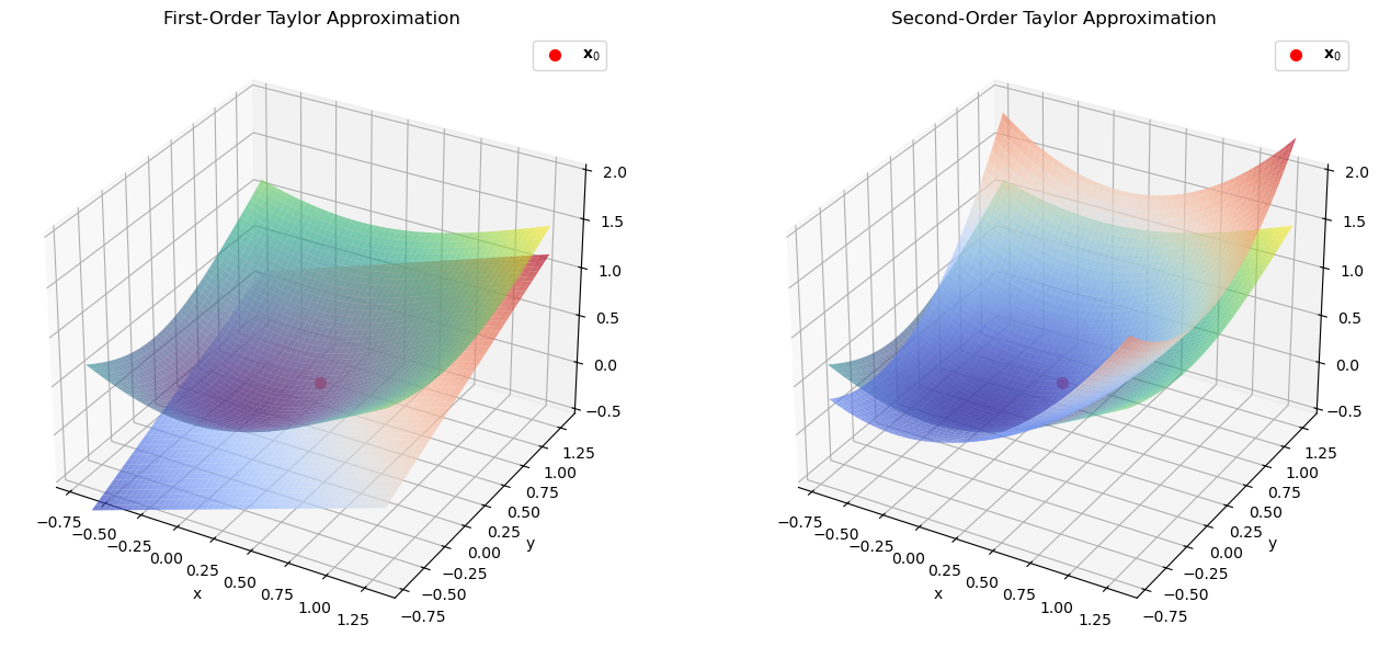
This visualization shows how the first-order (left) and second-order (right) Taylor expansions approximate the original function locally around the point \( (0.3,0.3) \), but deviates farther away. Both approximations are shown in blue to red and the original function in yellow to green colors.
Taylor’s Theorem in Multiple Variables#
Theorem (Taylor’s Theorem in Multiple Variables (Second-Order Remainder))
Let \(f: \mathbb{R}^d \to \mathbb{R}\) be a function that is three times continuously differentiable on an open set \(U \subset \mathbb{R}^d\). Let \(\mathbf{x}_0 \in U\), and let \(\mathbf{x} \in U\) be such that the line segment between \(\mathbf{x}_0\) and \(\mathbf{x}\) lies entirely in \(U\). Then:
for some point \(\boldsymbol{\xi}\) on the open segment between \(\mathbf{x}_0\) and \(\mathbf{x}\).
This is the first-order Taylor approximation with remainder in integral form or mean value form.
We observe:
We’re approximating \(f(\mathbf{x})\) using only the first-order derivative, but the error (or remainder) is controlled by the second-order derivative, specifically involving the Hessian at some intermediate point \(\boldsymbol{\xi}\).
Therefore, it’s a first-order approximation with a second-order remainder.
Theorem (Taylor’s Theorem in Multiple Variables (Third-Order Integral Remainder))
Let \(f: \mathbb{R}^d \to \mathbb{R}\) be four times continuously differentiable on an open set \(U \subset \mathbb{R}^d\), and let \(\mathbf{x}_0, \mathbf{x} \in U\) such that the line segment between them lies entirely in \(U\). Then:
for some \(\boldsymbol{\xi}\) on the segment between \(\mathbf{x}_0\) and \(\mathbf{x}\).
Notes on Higher-Order Remainders
The third-order term involves a third-order tensor (all third partial derivatives), and the remainder is often written using multi-index notation or tensor contraction.
For applications in optimization and machine learning, most practical Taylor approximations stop at second-order, because third- and higher-order terms are expensive to compute and rarely needed unless using higher-order optimization methods.
Theorem (Big-O Remainder in Multivariable Case)
For \(f: \mathbb{R}^d \to \mathbb{R}\), we can write:
Where:
\(\alpha \in \mathbb{N}^d\) is a multi-index,
\(D^\alpha f\) is the partial derivative corresponding to \(\alpha\),
\((\mathbf{x} - \mathbf{x}_0)^\alpha = \prod_i (x_i - x_{0,i})^{\alpha_i}\),
And \(|\alpha| = \sum_i \alpha_i\).
The exact form (Lagrange or integral remainder) gives precise values, but is often impractical.
The Big-O remainder focuses on how the error behaves, not what it is exactly.
This is especially useful in:
Error estimates
Convergence analysis
Algorithm design (e.g. gradient descent, Newton’s method)
While we can state and prove Taylor’s theorem for a remainder of arbitrary order, we prove only the version of the theorem for the first order Taylor expansion with second-order remainder.
Proof. Proof Sketch (Mean Value Form of the Remainder)
Let’s define the path:
This is a straight-line path from \(\mathbf{x}_0\) to \(\mathbf{x}\).
Define the composite function \(g(t) = f(\gamma(t))\). Then \(g : [0,1] \to \mathbb{R}\) is a function of one variable.
Using the chain rule, we have:
and
Now apply the Taylor expansion of \(g(t)\) around \(t = 0\) with Lagrange remainder (from single-variable calculus):
Substitute back:
\(g(0) = f(\mathbf{x}_0)\)
\(g'(0) = \nabla f(\mathbf{x}_0)^T (\mathbf{x} - \mathbf{x}_0)\)
\(g''(\tau) = (\mathbf{x} - \mathbf{x}_0)^T \nabla^2 f(\gamma(\tau)) (\mathbf{x} - \mathbf{x}_0)\)
So:
where \(\boldsymbol{\xi} = \gamma(\tau)\) lies on the open segment between \(\mathbf{x}_0\) and \(\mathbf{x}\).
Q.E.D.
🔍 Summary#
Expansion Type |
Uses |
Remainder Involves |
|---|---|---|
First-order |
\(f, \nabla f\) at \(\mathbf{x}_0\) |
Second derivatives (Hessian) |
Second-order |
\(f, \nabla f, \nabla^2 f\) at \(\mathbf{x}_0\) |
Third derivatives |
Outlook#
A nice property of second-order Taylor expansion is that the resulting function is a quadratic and that we know how to analytically solve quadratic optimization problems. This observation is the key idea behind Newton’s method. Thus, similarly to how linear approximation using the gradient (a.k.a. first-order Taylor expansion) was the basis for first-order optimization, the second order Taylor expansion will be the basis for second-order optimization methods. However, before we delve into second-order optimization, we have to study the properties of matrices such as the Hessian at a deeper level.