Second Order Condition for Minima

We have seen that first-order information (i.e. the gradient) is insufficient to characterize local minima. But we can say more with second-order information (i.e. the Hessian).

First we prove a necessary second-order condition for local minima.

Proposition (Necessary Second-Order Condition for Local Minima)

If \(\mathbf{x}^*\) is a local minimum of \(f\) and \(f\) is twice continuously differentiable in a neighborhood of \(\mathbf{x}^*\), then \(\nabla^2 f(\mathbf{x}^*)\) is positive semi-definite.

Proof. Let \(\mathbf{x}^*\) be a local minimum of \(f\), and suppose towards a contradiction that \(\nabla^2 f(\mathbf{x}^*)\) is not positive semi-definite.

Let \(\mathbf{h}\) be such that \(\mathbf{h}^{\!\top\!}\nabla^2 f(\mathbf{x}^*)\mathbf{h} < 0\), noting that by the continuity of \(\nabla^2 f\) we have

\[\lim_{t \to 0} \nabla^2 f(\mathbf{x}^* + t\mathbf{h}) = \nabla^2 f(\mathbf{x}^*)\]

Hence

\[\lim_{t \to 0} \mathbf{h}^{\!\top\!}\nabla^2 f(\mathbf{x}^* + t\mathbf{h})\mathbf{h} = \mathbf{h}^{\!\top\!}\nabla^2 f(\mathbf{x}^*)\mathbf{h} < 0\]

Thus there exists \(T > 0\) such that \(\mathbf{h}^{\!\top\!}\nabla^2 f(\mathbf{x}^* + t\mathbf{h})\mathbf{h} < 0\) for all \(t \in [0,T]\).

Now we apply Taylor’s theorem: for any \(t \in (0,T]\), there exists \(t' \in (0,t)\) such that

\[f(\mathbf{x}^* + t\mathbf{h}) = f(\mathbf{x}^*) + \underbrace{t\mathbf{h}^{\!\top\!}\nabla f(\mathbf{x}^*)}_0 + \frac{1}{2}t^2\mathbf{h}^{\!\top\!}\nabla^2 f(\mathbf{x}^* + t'\mathbf{h})\mathbf{h} < f(\mathbf{x}^*)\]

where the middle term vanishes because \(\nabla f(\mathbf{x}^*) = \mathbf{0}\) by the previous result.

It follows that \(\mathbf{x}^*\) is not a local minimum, a contradiction. Hence \(\nabla^2 f(\mathbf{x}^*)\) is positive semi-definite. ◻

Now we give sufficient conditions for local minima.

Proposition (Sufficient Second-Order Condition for Local Minima)

Suppose \(f\) is twice continuously differentiable with \(\nabla^2 f\) positive semi-definite in a neighborhood of \(\mathbf{x}^*\), and that \(\nabla f(\mathbf{x}^*) = \mathbf{0}\).

Then \(\mathbf{x}^*\) is a local minimum of \(f\).

Furthermore if \(\nabla^2 f(\mathbf{x}^*)\) is positive definite, then \(\mathbf{x}^*\) is a strict local minimum.

Proof. Let \(B\) be an open ball of radius \(r > 0\) centered at \(\mathbf{x}^*\) which is contained in the neighborhood.

Applying Taylor’s theorem, we have that for any \(\mathbf{h}\) with \(\|\mathbf{h}\|_2 < r\), there exists \(t \in (0,1)\) such that

\[f(\mathbf{x}^* + \mathbf{h}) = f(\mathbf{x}^*) + \underbrace{\mathbf{h}^{\!\top\!}\nabla f(\mathbf{x}^*)}_0 + \frac{1}{2}\mathbf{h}^{\!\top\!}\nabla^2 f(\mathbf{x}^* + t\mathbf{h})\mathbf{h} \geq f(\mathbf{x}^*)\]

The last inequality holds because \(\nabla^2 f(\mathbf{x}^* + t\mathbf{h})\) is positive semi-definite (since \(\|t\mathbf{h}\|_2 = t\|\mathbf{h}\|_2 < \|\mathbf{h}\|_2 < r\)), so \(\mathbf{h}^{\!\top\!}\nabla^2 f(\mathbf{x}^* + t\mathbf{h})\mathbf{h} \geq 0\).

Since \(f(\mathbf{x}^*) \leq f(\mathbf{x}^* + \mathbf{h})\) for all directions \(\mathbf{h}\) with \(\|\mathbf{h}\|_2 < r\), we conclude that \(\mathbf{x}^*\) is a local minimum.

Now further suppose that \(\nabla^2 f(\mathbf{x}^*)\) is strictly positive definite.

Since the Hessian is continuous we can choose another ball \(B'\) with radius \(r' > 0\) centered at \(\mathbf{x}^*\) such that \(\nabla^2 f(\mathbf{x})\) is positive definite for all \(\mathbf{x} \in B'\).

Then following the same argument as above (except with a strict inequality now since the Hessian is positive definite) we have \(f(\mathbf{x}^* + \mathbf{h}) > f(\mathbf{x}^*)\) for all \(\mathbf{h}\) with \(0 < \|\mathbf{h}\|_2 < r'\). Hence \(\mathbf{x}^*\) is a strict local minimum. ◻

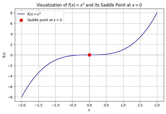
Note that, perhaps counterintuitively, the conditions \(\nabla f(\mathbf{x}^*) = \mathbf{0}\) and \(\nabla^2 f(\mathbf{x}^*)\) positive semi-definite are not enough to guarantee a local minimum at \(\mathbf{x}^*\)!

Consider the function \(f(x) = x^3\). We have \(f'(0) = 0\) and \(f''(0) = 0\) (so the Hessian, which in this case is the \(1 \times 1\) matrix \(\begin{bmatrix}0\end{bmatrix}\), is positive semi-definite). However, \(f\) has a saddle point at \(x = 0\):

Show code cell source Hide code cell source

import numpy as np
import matplotlib.pyplot as plt

x = np.linspace(-2, 2, 400)
y = x**3

plt.figure(figsize=(8, 5))
plt.plot(x, y, label=r'$f(x) = x^3$', color='blue')
plt.scatter(0, 0, color='red', s=80, zorder=5, label='Saddle point at $x=0$')
plt.axhline(0, color='gray', linewidth=0.8, linestyle='--')
plt.axvline(0, color='gray', linewidth=0.8, linestyle='--')
plt.title(r'Visualization of $f(x) = x^3$ and its Saddle Point at $x=0$')
plt.xlabel('$x$')
plt.ylabel('$f(x)$')
plt.legend()
plt.grid(True)
plt.show()

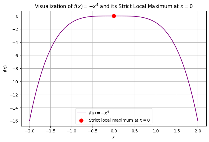
The function \(f(x) = -x^4\) is an even worse offender – it has the same gradient and Hessian at \(x = 0\), but \(x = 0\) is a strict local maximum for this function!

Show code cell source Hide code cell source

import numpy as np
import matplotlib.pyplot as plt

x = np.linspace(-2, 2, 400)
y = -x**4

plt.figure(figsize=(8, 5))
plt.plot(x, y, label=r'$f(x) = -x^4$', color='purple')
plt.scatter(0, 0, color='red', s=80, zorder=5, label='Strict local maximum at $x=0$')
plt.axhline(0, color='gray', linewidth=0.8, linestyle='--')
plt.axvline(0, color='gray', linewidth=0.8, linestyle='--')
plt.title(r'Visualization of $f(x) = -x^4$ and its Strict Local Maximum at $x=0$')
plt.xlabel('$x$')
plt.ylabel('$f(x)$')
plt.legend()
plt.grid(True)
plt.show()

For these reasons we require that the Hessian remains positive semi-definite as long as we are close to \(\mathbf{x}^*\).

Unfortunately, this condition is not practical to check computationally, but in some cases we can verify it analytically (usually by showing that \(\nabla^2 f(\mathbf{x})\) is p.s.d. for all \(\mathbf{x} \in \mathbb{R}^d\)).

Also, if \(\nabla^2 f(\mathbf{x}^*)\) is strictly positive definite, the continuity assumption on \(f\) implies this condition, so we don’t have to worry.