Functions of Random Variables#
A very useful property of random variables is that functions of random variables are again random variables.
Formal Definition of a Function of a Random Variable#
Let \(X : \Omega \to \mathbb{R}\) be a random variable, and let \(f : \mathbb{R} \to \mathbb{R}\) be a deterministic function. Then the composition \(Y = f(X)\) defines a new random variable:
This is again measurable and hence a valid random variable.
Example: Square of a Random Variable#
Suppose \(X\) is the number of heads in two tosses of a fair coin, with range \(X(\Omega) = \{0, 1, 2\}\). Let \(Y = f(X) = X^2\). Then
We can compute the distribution of \(Y\) by mapping the probabilities from \(X\) through \(f\):
So even though the function \(f(x) = x^2\) changes the values, it preserves how probabilities are transported.
General Recipe#
To compute the distribution of \(Y = f(X)\), use:
Discrete case:
\[\begin{split} \mathbb{P}(Y = y) = \sum_{\substack{x \in X(\Omega) \\ f(x) = y}} \mathbb{P}(X = x) \end{split}\]Continuous case (if \(f\) is invertible and differentiable): Use the change-of-variable formula for densities:
Theorem (Change of Variable Formula)
Let \(X\) be a continuous random variable with probability density function (PDF) \(p_X(x)\).
Let \(Y = f(X)\) be a new random variable, where \(f\) is an invertible and differentiable function.
Then the PDF of \(Y\) is given by:
Proof. Change of Variable Formula
Let \(X\) be a continuous random variable with probability density function (PDF) \(p_X(x)\), and let \(Y = f(X)\) be a new random variable, where \(f\) is an invertible and differentiable function.
We want to find the PDF of \(Y\), denoted as \(p_Y(y)\).
The proof starts from the definition of the CDF of \(Y\), which is \(F_Y(y) = P(Y \le y)\).
The PDF can then be found by differentiating the CDF: \(p_Y(y) = \frac{d}{dy}F_Y(y)\).
We will consider two cases for the function \(f\): monotonically increasing and monotonically decreasing.
Case 1: \(f\) is strictly monotonically increasing
If \(f\) is an increasing function, its inverse \(f^{-1}\) is also an increasing function.
The inequality \(f(X) \le y\) is equivalent to \(X \le f^{-1}(y)\).
CDF of Y: The CDF of \(Y\) can be expressed in terms of the CDF of \(X\):
\[ F_Y(y) = P(Y \le y) = P(f(X) \le y) = P(X \le f^{-1}(y)) = F_X(f^{-1}(y)) \]PDF of Y: To find the PDF of \(Y\), we differentiate its CDF with respect to \(y\).
Using the chain rule, we get:
\[ p_Y(y) = \frac{d}{dy}F_Y(y) = \frac{d}{dy}F_X(f^{-1}(y)) \]The derivative of \(F_X(x)\) is \(p_X(x)\), so:
\[ p_Y(y) = p_X(f^{-1}(y)) \cdot \frac{d}{dy}f^{-1}(y) \]Since \(f\) (and thus \(f^{-1}\)) is increasing, its derivative \(\frac{d}{dy}f^{-1}(y)\) is positive.
Therefore, we can write it as an absolute value:
\[ p_Y(y) = p_X(f^{-1}(y)) \cdot \left| \frac{d}{dy}f^{-1}(y) \right| \]
Case 2: \(f\) is strictly monotonically decreasing
If \(f\) is a decreasing function, its inverse \(f^{-1}\) is also a decreasing function.
The inequality \(f(X) \le y\) is now equivalent to \(X \ge f^{-1}(y)\).
CDF of Y: The CDF of \(Y\) is:
\[ F_Y(y) = P(Y \le y) = P(f(X) \le y) = P(X \ge f^{-1}(y)) \]For a continuous variable, \(P(X \ge x) = 1 - P(X < x) = 1 - P(X \le x) = 1 - F_X(x)\).
So:
\[ F_Y(y) = 1 - F_X(f^{-1}(y)) \]PDF of Y: Differentiating the CDF of \(Y\) with respect to \(y\):
\[ p_Y(y) = \frac{d}{dy}F_Y(y) = \frac{d}{dy}(1 - F_X(f^{-1}(y))) = - \frac{d}{dy}F_X(f^{-1}(y)) \]Using the chain rule again:
\[ p_Y(y) = - p_X(f^{-1}(y)) \cdot \frac{d}{dy}f^{-1}(y) \]Since \(f\) (and thus \(f^{-1}\)) is decreasing, its derivative \(\frac{d}{dy}f^{-1}(y)\) is negative.
The negative sign in the expression makes the whole term positive, as a PDF must be. We can express this using an absolute value:
\[ p_Y(y) = p_X(f^{-1}(y)) \cdot \left| \frac{d}{dy}f^{-1}(y) \right| \]
Conclusion
In both cases—whether \(f\) is monotonically increasing or decreasing—the formula for the PDF of \(Y\) is the same:
This completes the proof for any invertible and differentiable function \(f\).
Example: Exponential Distribution#
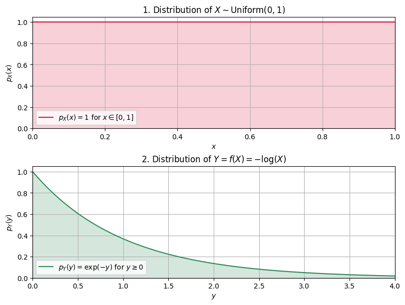
Let \(X \sim \text{Uniform}(0, 1)\), and let \(Y = f(X) = -\log(X)\).
Let’s plot the function \(f(x) = -log(x)\):
Show code cell source
import numpy as np
import matplotlib.pyplot as plt

# Define the function f and its inverse
f = lambda x: -np.log(x)
f_inv = lambda y: np.exp(-y)
x_vals = np.linspace(0.01, 1.0, 500)  # avoid log(0)
y_vals = f(x_vals)

y_vals_inv = f_inv(y_vals)

# Plot the function f(x) = -log(x)
plt.figure(figsize=(8, 4))
plt.plot(x_vals, y_vals, color='darkorange', label='f(x) = -log(x)')
plt.xlabel('x')
plt.ylabel('f(x)')
plt.title('Function: f(x) = -log(x)')
plt.xlim(0, 1)
plt.ylim(0, 4)
plt.grid(True)
# plt.legend()
plt.show()
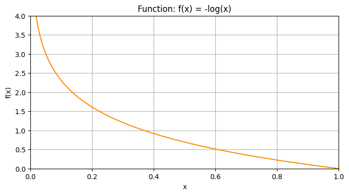
We see that \(f(x) = -log(x)\) is a strictly monotonically increasing function and that all \(f(x)\) are positive.
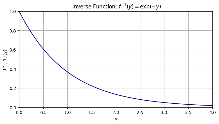
To apply the change of variable formula, we need to find the inverse of \(f\):
Let’s plot the inverse function \(f^{-1}(y) = \exp(-y)\) and the PDF of \(Y\):
Show code cell source
import numpy as np
import matplotlib.pyplot as plt

# Define the function f and its inverse
f = lambda x: -np.log(x)
f_inv = lambda y: np.exp(-y)
x_vals = np.linspace(0.01, 1.0, 500)  # avoid log(0)
y_vals = f(x_vals)

y_vals_inv = f_inv(y_vals)

# Plot the function f(x) = -log(x)
plt.figure(figsize=(8, 4))
# plt.plot(x_vals, y_vals, color='darkorange', label='f(x) = -log(x)')
plt.xlabel('y')
plt.ylabel('f^{-1}(y)')
plt.title(' Inverse Function: $f^{-1}(y) = \\exp(-y)$')
plt.plot(y_vals,y_vals_inv, color='darkblue')
plt.xlim(0, 4)
plt.ylim(0, 1)
plt.grid(True)
# plt.legend()
plt.show()
We can now use the change of variable formula to find the PDF of \(Y\):
We know that for \(y \in [0, \infty)\), \(f^{-1}(y) \in [0, 1]\) and \(X \sim \text{Uniform}(0, 1)\), so \(p_X(f^{-1}(y)) = 1\) for \(y \in [0, \infty)\).
We also know that \(\frac{d}{dy} \exp(-y) = -\exp(-y)\).
Thus, we can write:
To conclude, we can write the PDF of \(Y\) as:
We can now plot the PDF of \(Y\) and compare it to the PDF of \(X\):
Show code cell source
import numpy as np
import matplotlib.pyplot as plt
from scipy.stats import uniform

# Define the function f and its inverse
f = lambda x: -np.log(x)
f_inv = lambda y: np.exp(-y)
x_vals = np.linspace(0.0001, 1.0, 500)  # avoid log(0)
y_vals = f(x_vals)

# PDF of X ~ Uniform(0,1)
pdf_X = uniform.pdf(x_vals, loc=0, scale=1)

# PDF of Y using change-of-variables
y_range = np.linspace(0.0, 4.0, 500)
pdf_Y = uniform.pdf(f_inv(y_range), loc=0, scale=1) * np.abs(-f_inv(y_range))

# Create the figure again with corrected labels
fig, axs = plt.subplots(2, 1, figsize=(8, 6), constrained_layout=True)

# 2. Plot the distribution of X
axs[0].plot(x_vals, pdf_X, color='crimson', label='$p_X(x) = 1$ for $x \\in [0,1]$')
axs[0].fill_between(x_vals, pdf_X, alpha=0.2, color='crimson')
axs[0].set_title("1. Distribution of $X \\sim \\mathrm{Uniform}(0,1)$")
axs[0].set_xlabel('$x$')
axs[0].set_ylabel('$p_X(x)$')
axs[0].set_xlim(0, 1)
axs[0].set_ylim(0, 1.05)
axs[0].grid(True)
axs[0].legend(loc='lower left')

# 3. Plot the distribution of Y = f(X)
axs[1].plot(y_range, pdf_Y, color='seagreen', label='$p_Y(y) = \\exp(-y)$ for $y \\geq 0$')
axs[1].fill_between(y_range, pdf_Y, alpha=0.2, color='seagreen')
axs[1].set_title("2. Distribution of $Y = f(X) = -\\log(X)$")
axs[1].set_xlabel('$y$')
axs[1].set_ylabel('$p_Y(y)$')
axs[1].set_xlim(0, 4)
axs[1].set_ylim(0, 1.05)
axs[1].grid(True)
axs[1].legend(loc='lower left')

plt.show()