Matrix Norms

Matrix Norms#

Matrix norms provide a way to measure the “size” or “magnitude” of a matrix. They are used throughout machine learning and numerical analysis—for example, to quantify approximation error, assess convergence in optimization algorithms, or bound the spectral properties of linear transformations.

Definition#

A matrix norm is a function \( \|\cdot\| : \mathbb{R}^{m \times n} \to \mathbb{R} \) satisfying the following properties for all matrices \( \mathbf{A}, \mathbf{B} \in \mathbb{R}^{m \times n} \) and all scalars \( \alpha \in \mathbb{R} \):

Non-negativity: \( \|\mathbf{A}\| \geq 0 \)
Definiteness: \( \|\mathbf{A}\| = 0 \iff \mathbf{A} = 0 \)
Homogeneity: \( \|\alpha \mathbf{A}\| = |\alpha| \cdot \|\mathbf{A}\| \)
Triangle inequality: \( \|\mathbf{A} + \mathbf{B}\| \leq \|\mathbf{A}\| + \|\mathbf{B}\| \)

These are the minimal axioms for a matrix norm — analogous to vector norms.

Common Matrix Norms#

1. Frobenius Norm#

Defined by:

\[ \|\mathbf{A}\|_F = \sqrt{\sum_{i,j} A_{ij}^2} = \sqrt{\mathrm{tr}(\mathbf{A}^\top \mathbf{A})} \]

It treats the matrix as a vector in \( \mathbb{R}^{mn} \).

2. Induced (Operator) Norms#

Given a vector norm \( \|\cdot\| \), the induced matrix norm is:

\[ \|\mathbf{A}\| = \sup_{\mathbf{x} \neq 0} \frac{\|\mathbf{A} \mathbf{x}\|}{\|\mathbf{x}\|} = \sup_{\|\mathbf{x}\| = 1} \|\mathbf{A} \mathbf{x}\| \]

Examples:

Spectral norm: Induced by the Euclidean norm \( \|\cdot\|_2 \).

Equal to the largest singular value of \( \mathbf{A}. \)
\( \ell_1 \) norm: Maximum absolute column sum.
\( \ell_\infty \) norm: Maximum absolute row sum.

Submultiplicativity#

The submultiplicative property is an additional structure, not a required axiom. Many useful matrix norms (especially induced norms) do satisfy it, but not all matrix norms do.

When a matrix norm satisfies it, we say it is a:

Submultiplicative matrix norm

Induced norms satisfy the submultiplicative property:

\[ \|\mathbf{A}\mathbf{B}\| \leq \|\mathbf{A}\| \cdot \|\mathbf{B}\| \]

For the Frobenius norm:

\[ \|\mathbf{A}\mathbf{B}\|_F \leq \|\mathbf{A}\|_F \cdot \|\mathbf{B}\|_F \]

Norm	Submultiplicative?	Notes
Frobenius norm \(\|\cdot\|_F\)	✅ Yes	But not induced from a vector norm
Induced norms (e.g., spectral)	✅ Yes	Always submultiplicative
Entrywise max norm	❌ No	Not submultiplicative in general

All norms on a finite-dimensional vector space are equivalent (they define the same topology), but may differ in scaling.

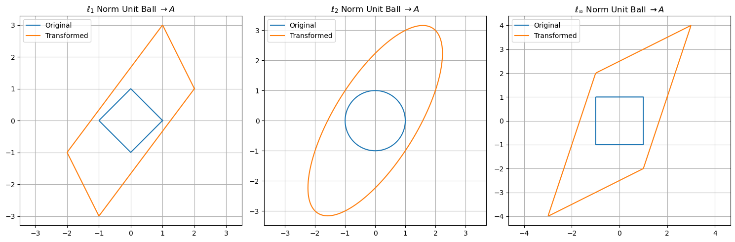
Visual Comparison (2D case)#

In 2D, vector norms induce different geometries:

\( \ell_2 \): circular level sets
\( \ell_1 \): diamond-shaped level sets
\( \ell_\infty \): square level sets

This influences which directions are favored in optimization and which vectors are “small” under a given norm.

Here is a visual comparison of how different induced norms transform unit circles in 2D space under a linear transformation defined by a matrix \( A \):

\[\begin{split} \mathbf{A} = \begin{bmatrix} 2 & 1 \\ 1 & 3 \end{bmatrix} \end{split}\]

../_images/2e624506e358285f71d98488340f85414b516a93b19be5e5ba1dd94bed7d8ae7.png

Let’s give formal definitions and proofs for several commonly used induced matrix norms, also known as operator norms, derived from vector norms.

Let \(\|\cdot\|\) be a vector norm on \(\mathbb{R}^n\), and define the induced matrix norm for \(\mathbf{A} \in \mathbb{R}^{m \times n}\) as:

\[ \|\mathbf{A}\| = \sup_{\mathbf{x} \neq 0} \frac{\|\mathbf{A} \mathbf{x}\|}{\|\mathbf{x}\|} = \sup_{\|\mathbf{x}\| = 1} \|\mathbf{A} \mathbf{x}\| \]

We’ll now state and prove specific formulas for induced norms when the underlying vector norm is:

\(\ell_1\)
\(\ell_\infty\)
\(\ell_2\) (spectral norm)

1. Induced \(\ell_1\) Norm#

Claim: If \(\|\mathbf{x}\| = \|\mathbf{x}\|_1\), then:

\[ \|\mathbf{A}\|_1 = \max_{1 \leq j \leq n} \sum_{i=1}^m |A_{ij}| \quad \text{(maximum absolute column sum)} \]

Proof. Let \(\mathbf{A} = [a_{ij}] \in \mathbb{R}^{m \times n}\).

Then by the definition of the induced norm:

\[ \|\mathbf{A}\|_1 = \sup_{\|\mathbf{x}\|_1 = 1} \|\mathbf{A} \mathbf{x}\|_1 = \sup_{\|\mathbf{x}\|_1 = 1} \sum_{i=1}^m \left| \sum_{j=1}^n a_{ij} x_j \right| \]

Apply the triangle inequality inside the absolute value:

\[ \leq \sup_{\|\mathbf{x}\|_1 = 1} \sum_{i=1}^m \sum_{j=1}^n |a_{ij}| \cdot |x_j| = \sup_{\|\mathbf{x}\|_1 = 1} \sum_{j=1}^n |x_j| \left( \sum_{i=1}^m |a_{ij}| \right) \]

Let us define the column sums:

\[ c_j := \sum_{i=1}^m |a_{ij}| \]

Then the expression becomes:

\[ \sum_{j=1}^n |x_j| c_j \leq \max_j c_j \cdot \sum_{j=1}^n |x_j| = \max_j c_j \]

since \(\sum_{j=1}^n |x_j| = \|\mathbf{x}\|_1 = 1\), and this is a convex combination of the \(c_j\).

Attainment of the Maximum

Let \(j^* \in \{1, \dots, n\}\) be the index of the column with maximum sum:

\[ c_{j^*} = \max_j \sum_i |a_{ij}| \]

Now choose the standard basis vector \(\mathbf{e}_{j^*} \in \mathbb{R}^n\), where:

\[\begin{split} (\mathbf{e}_{j^*})_j = \begin{cases} 1, & j = j^* \\\\ 0, & j \neq j^* \end{cases} \end{split}\]

Then \(\|\mathbf{e}_{j^*}\|_1 = 1\), and:

\[ \|\mathbf{A} \mathbf{e}_{j^*}\|_1 = \sum_{i=1}^m \left| a_{i j^*} \right| = c_{j^*} \]

So the upper bound is achieved, and we conclude:

\[ \|\mathbf{A}\|_1 = \max_j \sum_i |a_{ij}| \]

QED.

2. Induced \(\ell_\infty\) Norm#

Claim: If \(\|\mathbf{x}\| = \|\mathbf{x}\|_\infty\), then:

\[ \|\mathbf{A}\|_\infty = \max_{1 \leq i \leq m} \sum_{j=1}^n |A_{ij}| \quad \text{(maximum absolute row sum)} \]

Proof. Let \(\|\mathbf{x}\|_\infty = 1\).

Then:

\[ \|A \mathbf{x}\|_\infty = \max_{i} \left| \sum_j a_{ij} x_j \right| \leq \max_i \sum_j |a_{ij}||x_j| \leq \max_i \sum_j |a_{ij}| \]

Equality is achieved by choosing \(x_j = \operatorname{sign}(a_{ij^*})\) at the row \(i^*\) with largest sum. So:

\[ \|\mathbf{A}\|_\infty = \max_i \sum_j |a_{ij}| \]

QED.

3. Induced \(\ell_2\) Norm (Spectral Norm)#

Claim: If \(\|\cdot\| = \|\cdot\|_2\), then:

\[ \|\mathbf{A}\|_2 = \sigma_{\max}(\mathbf{A}) = \sqrt{\lambda_{\max}(\mathbf{A}^\top \mathbf{A})} \]

where \(\sigma_{\max}(\mathbf{A})\) is the largest singular value of \(\mathbf{A}\), and \(\lambda_{\max}\) denotes the largest eigenvalue.

Proof. Let \(\|\mathbf{x}\|_2 = 1\).

Then:

\[ \|\mathbf{A}\|_2 = \sup_{\|\mathbf{x}\|_2 = 1} \|\mathbf{A} \mathbf{x}\|_2 = \sup_{\|\mathbf{x}\|_2 = 1} \sqrt{(\mathbf{A} \mathbf{x})^\top (\mathbf{A} \mathbf{x})} = \sup_{\|\mathbf{x}\|_2 = 1} \sqrt{\mathbf{x}^\top \mathbf{A}^\top \mathbf{A} \mathbf{x}} \]

This is the Rayleigh quotient of \(\mathbf{A}^\top \mathbf{A}\), a symmetric PSD matrix.

So:

\[ \|\mathbf{A}\|_2 = \sqrt{\lambda_{\max}(\mathbf{A}^\top \mathbf{A})} \]

QED.

Summary Table#

Vector Norm	Induced Matrix Norm
\(\ell_1\)	Max column sum:	\(\max_j \sum_i a_{ij}\)
\(\ell_\infty\)	Max row sum:	\(\max_i \sum_j a_{ij}\)
\(\ell_2\)	Largest singular value:	\(\sqrt{\lambda_{\max}(A^\top A)}\)

Applications in Machine Learning#

In optimization, norms define constraints (e.g., Lasso uses \( \ell_1 \)-norm penalty).
In regularization, norms quantify complexity of parameter matrices (e.g., weight decay with \( \ell_2 \)-norm).
In spectral methods, matrix norms bound approximation error (e.g., spectral norm bounds for generalization).

Collaborative Filtering and Matrix Factorization#

Collaborative filtering is a foundational technique in recommendation systems, where the goal is to predict a user’s preference for items based on observed interactions (such as ratings, clicks, or purchases). The key assumption underlying collaborative filtering is that user preferences and item characteristics lie in a shared low-dimensional latent space. That is, although we observe only sparse user-item interactions, there exists a hidden structure — often of low rank — that explains these patterns.

A common model formalizes this intuition by representing the user-item rating matrix \(R \in \mathbb{R}^{m \times n}\) as the product of two low-rank matrices:

\[ R \approx UV^\top \]

where \(U \in \mathbb{R}^{m \times k}\) encodes latent user features and \(V \in \mathbb{R}^{n \times k}\) encodes latent item features, for some small \(k \ll \min(m, n)\). The model is typically fit by minimizing the squared error over observed entries, together with regularization to prevent overfitting:

\[ \min_{U, V} \sum_{(i,j) \in \Omega} (R_{ij} - U_i^\top V_j)^2 + \lambda (\|U\|_F^2 + \|V\|_F^2) \]

where \(\Omega \subset [m] \times [n]\) is the set of observed ratings, and \(\| \cdot \|_F\) is the Frobenius norm. This formulation implicitly assumes that missing ratings are missing at random and that users with similar latent profiles tend to rate items similarly — an assumption that allows the model to generalize from sparse data.

class MatrixFactorization:
    def __init__(self, k=2, steps=1000, lam=0.1):
        """
        Initializes the matrix factorization model.

        Parameters:
        - k (int): number of latent features
        - steps (int): number of ALS iterations
        - lam (float): regularization strength
        """
        self.k = k
        self.steps = steps
        self.lam = lam
        self.U = None
        self.V = None

    def fit(self, R, mask):
        """
        Fit the model to the observed rating matrix using ALS.

        Parameters:
        - R (ndarray): observed rating matrix (with zeros for missing entries)
        - mask (ndarray): boolean matrix where True indicates an observed entry
        """
        num_users, num_items = R.shape
        self.U = np.random.randn(num_users, self.k)
        self.V = np.random.randn(num_items, self.k)

        for step in range(self.steps):
            # Update U
            for i in range(num_users):
                V_masked = self.V[mask[i, :]]
                R_i = R[i, mask[i, :]]
                if len(R_i) > 0:
                    A = V_masked.T @ V_masked + self.lam * np.eye(self.k)
                    b = V_masked.T @ R_i
                    self.U[i] = np.linalg.solve(A, b)
            # Update V
            for j in range(num_items):
                U_masked = self.U[mask[:, j]]
                R_j = R[mask[:, j], j]
                if len(R_j) > 0:
                    A = U_masked.T @ U_masked + self.lam * np.eye(self.k)
                    b = U_masked.T @ R_j
                    self.V[j] = np.linalg.solve(A, b)

    def predict(self):
        """
        Returns the full reconstructed rating matrix.
        """
        return self.U @ self.V.T

    def predict_single(self, user_idx, item_idx):
        """
        Predict a single rating for a user-item pair.

        Parameters:
        - user_idx (int): index of the user
        - item_idx (int): index of the item

        Returns:
        - float: predicted rating
        """
        return self.U[user_idx] @ self.V[item_idx]

This example demonstrates collaborative filtering via matrix factorization using the Frobenius norm to minimize reconstruction error:

../_images/69251b8e250cc98683333f7491c384a361a7a5c0145d979e14d57682ef5a0443.png

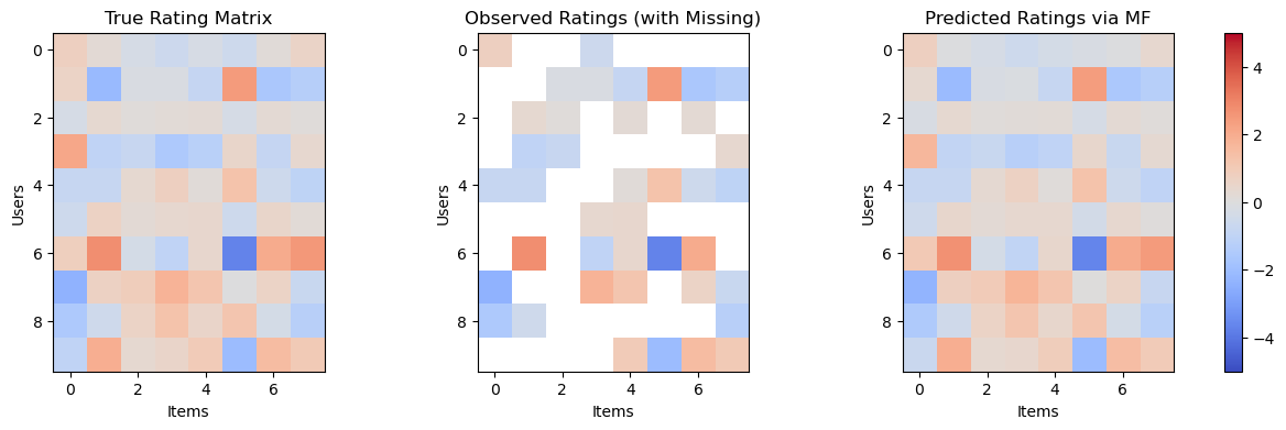
Left panel: The true user-item rating matrix (low-rank structure).
Middle panel: The observed entries, with ~50% missing.
Right panel: The matrix reconstructed via alternating least squares (ALS).

Matrix Norms

Contents

Matrix Norms#

Definition#

Common Matrix Norms#

1. Frobenius Norm#

2. Induced (Operator) Norms#

Submultiplicativity#

Visual Comparison (2D case)#

1. Induced \(\ell_1\) Norm#

Attainment of the Maximum

2. Induced \(\ell_\infty\) Norm#

3. Induced \(\ell_2\) Norm (Spectral Norm)#

Summary Table#

Applications in Machine Learning#

Collaborative Filtering and Matrix Factorization#