Orthogonal matrices#
A matrix \(\mathbf{Q} \in \mathbb{R}^{n \times n}\) is said to be orthogonal if its columns are pairwise orthonormal.
This definition implies that
or equivalently, \(\mathbf{Q}^{\!\top\!} = \mathbf{Q}^{-1}\).
A nice thing about orthogonal matrices is that they preserve inner products:
A direct result of this fact is that they also preserve 2-norms:
Therefore multiplication by an orthogonal matrix can be considered as a transformation that preserves length, but may rotate or reflect the vector about the origin.
Show code cell source
import numpy as np
import matplotlib.pyplot as plt

# Asymmetrical vector set
vectors = np.array([[1, 0.5, -0.5],
                    [0, 1, 0.5]])

# Orthogonal matrices
theta = np.pi / 4
Q_rot = np.array([[np.cos(theta), -np.sin(theta)],
                  [np.sin(theta),  np.cos(theta)]])
Q_reflect = np.array([[1, 0],
                      [0, -1]])

# Transform vectors
rotated_vectors = Q_rot @ vectors
reflected_vectors = Q_reflect @ vectors

# Unit square
square = np.array([[0, 1, 1, 0, 0],
                   [0, 0, 1, 1, 0]])
square_rotated = Q_rot @ square
square_reflected = Q_reflect @ square

# Plotting
fig, axes = plt.subplots(1, 3, figsize=(15, 5))

# Function to plot a frame
def plot_frame(ax, vecs, square, title, color):
    ax.quiver(np.zeros(vecs.shape[1]), np.zeros(vecs.shape[1]),
              vecs[0], vecs[1], angles='xy', scale_units='xy', scale=1, color=color)
    ax.plot(square[0], square[1], 'k--', lw=1.5, label='Transformed Unit Square')
    ax.fill(square[0], square[1], facecolor='lightgray', alpha=0.3)
    ax.set_title(title)
    ax.set_xlim(-2, 2)
    ax.set_ylim(-2, 2)
    ax.set_aspect('equal')
    ax.axhline(0, color='gray', lw=0.5)
    ax.axvline(0, color='gray', lw=0.5)
    ax.grid(True)
    ax.legend()

# Original
plot_frame(axes[0], vectors, square, "Original Vectors and Unit Square", 'blue')

# Rotation
plot_frame(axes[1], rotated_vectors, square_rotated, "Rotation (Orthogonal Q)", 'green')

# Reflection
plot_frame(axes[2], reflected_vectors, square_reflected, "Reflection (Orthogonal Q)", 'red')

plt.suptitle("Orthogonal Transformations: Vectors and Unit Square", fontsize=16)
plt.tight_layout(rect=[0, 0, 1, 0.93])
plt.show()
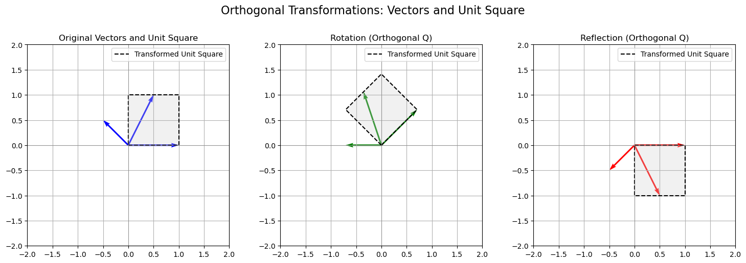
This enhanced visualization shows how orthogonal transformations affect both:
A set of asymmetric vectors, and
The unit square, which is preserved in shape and size but transformed in orientation:
Left: The original setup with vectors and the unit square.
Middle: A rotation — vectors and the square are rotated without distortion.
Right: A reflection — vectors and the square are flipped, but all lengths and angles remain unchanged.
✅ This highlights that orthogonal matrices are distance- and angle-preserving, making them key to rigid transformations like rotations and reflections.
Theorem (Determinant of an Orthogonal Matrix)
Let \(\mathbf{Q} \in \mathbb{R}^{n \times n}\) be an orthogonal matrix, meaning:
Then:
Proof. We start with the identity:
Now take the determinant of both sides:
Using the multiplicativity of determinants and the fact that \(\det(\mathbf{Q}^\top) = \det(\mathbf{Q})\) (since \(\det(\mathbf{A}^\top) = \det(\mathbf{A})\)):
Taking square roots:
Thus, the determinant of any orthogonal matrix is either \(+1\) (rotation) or \(-1\) (reflection).
\(\quad \blacksquare\)
🧠 Interpretation#
\(\det(\mathbf{Q}) = 1\): The transformation preserves orientation — e.g., rotation.
\(\det(\mathbf{Q}) = -1\): The transformation flips orientation — e.g., reflection.
This theorem is foundational in rigid body transformations, 3D graphics, PCA, and more.