Bayesian Inference for the Gaussian#
Let \(\mathbf{x} \in \mathbb{R}^d\) be drawn from a multivariate normal distribution with unknown mean \(\boldsymbol{\mu} \in \mathbb{R}^d\) and known covariance \(\boldsymbol{\Sigma}\):
We can write this distribution in exponential family form:
Rewriting this in exponential family form:
Where:
The natural parameter is: \(\boldsymbol{\eta} = \boldsymbol{\Sigma}^{-1} \boldsymbol{\mu}\)
The sufficient statistic is: \(T(\mathbf{x}) = \mathbf{x}\)
The log-partition function is: \(A(\boldsymbol{\eta}) = \frac{1}{2} \boldsymbol{\eta}^\top \boldsymbol{\Sigma} \boldsymbol{\eta}\)
The base measure is: \(h(\mathbf{x}) = \frac{1}{(2\pi)^{d/2} |\boldsymbol{\Sigma}|^{1/2}} \exp\left(-\frac{1}{2} \mathbf{x}^\top \boldsymbol{\Sigma}^{-1} \mathbf{x} \right)\)
Conjugate Prior for the Mean#
Given this exponential family form, the conjugate prior for the unknown mean \(\boldsymbol{\mu}\) (with fixed covariance \(\boldsymbol{\Sigma}\)) is a Gaussian prior:
This conjugate prior leads to a posterior distribution that is again Gaussian.
Derivation of the Posterior Distribution#
Given:
Observations: \(\mathbf{x}_1, \dots, \mathbf{x}_n \in \mathbb{R}^d\) i.i.d. from \(\mathbf{x}_i \sim \mathcal{N}(\boldsymbol{\mu}, \boldsymbol{\Sigma})\) with known covariance \(\boldsymbol{\Sigma}\) and unknown mean \(\boldsymbol{\mu}\)
Prior: \(\boldsymbol{\mu} \sim \mathcal{N}(\boldsymbol{\mu}_0, \boldsymbol{\Lambda}_0)\)
We want to compute the posterior distribution:
Step 1: Likelihood and Prior (log form)#
Log likelihood:#
Let \(\bar{\mathbf{x}} = \frac{1}{n} \sum_{i=1}^n \mathbf{x}_i\), then the sum of squared deviations becomes:
So up to constants:
Log prior:
Step 2: Posterior log density (unnormalized)#
Add log-prior and log-likelihood:
Step 3: Complete the Square#
We want to write the log posterior in the form:
To do this, combine the two quadratic terms:
Now we complete the square:
Let
Precision matrix:
\[ \boldsymbol{\Lambda}_n^{-1} = n \boldsymbol{\Sigma}^{-1} + \boldsymbol{\Lambda}_0^{-1} \]Mean:
\[ \boldsymbol{\mu}_n = \boldsymbol{\Lambda}_n \left(n \boldsymbol{\Sigma}^{-1} \bar{\mathbf{x}} + \boldsymbol{\Lambda}_0^{-1} \boldsymbol{\mu}_0 \right) \]
Then:
✅ Final Posterior#
The posterior is a Gaussian distribution:
With:
Posterior mean:
\[ \boldsymbol{\mu}_n = \left(n \boldsymbol{\Sigma}^{-1} + \boldsymbol{\Lambda}_0^{-1} \right)^{-1} \left(n \boldsymbol{\Sigma}^{-1} \bar{\mathbf{x}} + \boldsymbol{\Lambda}_0^{-1} \boldsymbol{\mu}_0 \right) \]Posterior covariance:
\[ \boldsymbol{\Lambda}_n = \left(n \boldsymbol{\Sigma}^{-1} + \boldsymbol{\Lambda}_0^{-1} \right)^{-1} \]
Interpretation#
The posterior is a weighted average of the prior mean \(\boldsymbol{\mu}_0\) and the sample mean \(\bar{\mathbf{x}}\).
The prior can be interpreted as encoding \(n_0\) pseudo-observations, where \(n_0 = \text{tr}(\boldsymbol{\Sigma} \boldsymbol{\Lambda}_0^{-1})\) heuristically reflects its strength.
When \(n \to \infty\), the posterior converges to the MLE.
When \(n = 0\), the posterior is the prior.
Visualizing Posterior Updates for \(\boldsymbol{\mu}\)#
Let’s visualize how the posterior distribution over the mean \(\boldsymbol{\mu}\) updates as we observe more data points from a 2D Gaussian with known covariance.
We will use a Gaussian prior with mean \(\boldsymbol{\mu}_0 = (0, 0)\) and covariance \(\boldsymbol{\Lambda}_0 = \mathbf{I}\).
We will generate 10 data points from a 2D Gaussian with known covariance \(\boldsymbol{\Sigma} = \begin{pmatrix} 0.5 & 0.2 \\ 0.2 & 1.0 \end{pmatrix}\).
Show code cell source
import numpy as np
import matplotlib.pyplot as plt
from matplotlib.patches import Ellipse

def draw_cov_ellipse(mean, cov, ax, n_std=2, **kwargs):
    """Draw an ellipse representing the covariance matrix."""
    eigvals, eigvecs = np.linalg.eigh(cov)
    order = eigvals.argsort()[::-1]
    eigvals, eigvecs = eigvals[order], eigvecs[:, order]

    angle = np.degrees(np.arctan2(*eigvecs[:, 0][::-1]))
    width, height = 2 * n_std * np.sqrt(eigvals)
    ellipse = Ellipse(xy=mean, width=width, height=height, angle=angle, **kwargs)
    ax.add_patch(ellipse)

def posterior_updates_viz():
    # Ground truth
    mu_true = np.array([2.0, -1.0])
    Sigma = np.array([[0.5, 0.2], [0.2, 1.0]])  # known covariance

    # Prior
    mu0 = np.array([0.0, 0.0])
    Lambda0 = np.eye(2)

    # Generate data
    n_points = 10
    X = np.random.multivariate_normal(mu_true, Sigma, size=n_points)

    fig, axes = plt.subplots(2, 5, figsize=(16, 6))
    axes = axes.flatten()

    for i in range(n_points):
        ax = axes[i]

        if i == 0:
            mu_n = mu0
            Lambda_n_inv = Lambda0
            Lambda_n = np.linalg.inv(Lambda_n_inv)
            title = "n = 0 (Prior)"
        else:
            X_i = X[:i]
            x_bar = np.mean(X_i, axis=0)
            Lambda_n_inv = np.linalg.inv(Lambda0) + i * np.linalg.inv(Sigma)
            Lambda_n = np.linalg.inv(Lambda_n_inv)
            mu_n = Lambda_n @ (np.linalg.inv(Lambda0) @ mu0 + i * np.linalg.inv(Sigma) @ x_bar)
            title = f"n = {i}"

        # Plot
        ax.scatter(X[:i, 0], X[:i, 1], c='black', s=20, label='Data')
        draw_cov_ellipse(mu_n, Lambda_n, ax, edgecolor='blue', lw=2, facecolor='none', label='Posterior')
        ax.scatter(*mu_true, color='green', label='True Mean', marker='x', s=100)
        ax.set_xlim(-2, 4)
        ax.set_ylim(-4, 2)
        ax.set_aspect('equal')
        ax.set_title(title)
        ax.grid(True)

        if i == 0:
            draw_cov_ellipse(mu0, Lambda0, ax, edgecolor='gray', lw=2, facecolor='none', label='Prior')

        if i == 5:
            ax.legend()

    plt.suptitle("Posterior Updates for Mean of 2D Gaussian", fontsize=16)
    plt.tight_layout()
    plt.show()

posterior_updates_viz()
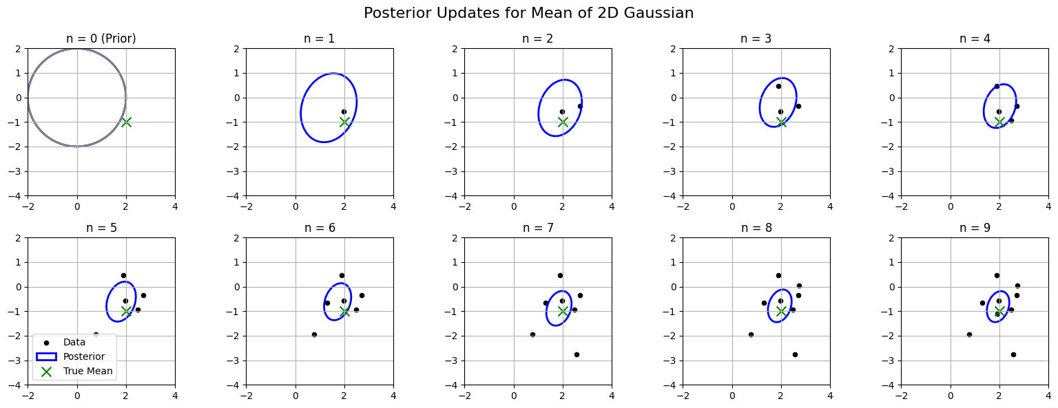
🧠 What You’ll See#
Prior ellipse centered at
mu0(0, 0)As each new data point is observed:
The posterior mean moves toward the true mean
The posterior uncertainty (ellipse size) shrinks
By \(n=10\), the posterior is tightly centered around the true mean
Bayesian Linear Regression#
Let’s derive Bayesian Linear Regression using:
A Gaussian prior on the weights: \(\mathbf{w} \sim \mathcal{N}(\mathbf{w}_0, \boldsymbol{\Lambda}_0)\)
A Gaussian likelihood for outputs: \(y_i \mid \mathbf{x}_i, \mathbf{w} \sim \mathcal{N}(\mathbf{x}_i^\top \mathbf{w}, \sigma^2)\)
The method of completing the square to compute the posterior over weights.
Setup: Likelihood and Prior#
Let:
\(\mathbf{X} \in \mathbb{R}^{n \times d}\): design matrix (rows are \(\mathbf{x}_i^\top\))
\(\mathbf{y} \in \mathbb{R}^n\): target vector
Likelihood#
The log-likelihood is (ignoring constants):
Prior#
Log prior:
🧠 Posterior (up to normalization)#
We combine the log prior and log likelihood:
We now complete the square to identify the posterior as a multivariate normal in \(\mathbf{w}\).
🧩 Completing the Square#
Expand each term:#
Likelihood term:
Prior term:
Combine terms:#
✅ Posterior Distribution#
This is the canonical form of a log-density of a Gaussian:
Hence the posterior is Gaussian:
Where:
Posterior covariance:
\[ \boxed{ \boldsymbol{\Lambda}_n = \left( \frac{1}{\sigma^2} \mathbf{X}^\top \mathbf{X} + \boldsymbol{\Lambda}_0^{-1} \right)^{-1} } \]Posterior mean:
\[ \boxed{ \mathbf{w}_n = \boldsymbol{\Lambda}_n \left( \frac{1}{\sigma^2} \mathbf{X}^\top \mathbf{y} + \boldsymbol{\Lambda}_0^{-1} \mathbf{w}_0 \right) } \]
📌 Interpretation#
If \(\boldsymbol{\Lambda}_0 = \tau^2 \mathbf{I}\) and \(\mathbf{w}_0 = \mathbf{0}\), this corresponds to ridge regression with \(\ell_2\) penalty \(\propto \frac{1}{\tau^2}\).
The prior acts as a regularizer, pulling weights toward \(\mathbf{w}_0\).
If \(n \to \infty\), the posterior converges to the MLE solution.
If \(n = 0\), the posterior equals the prior.
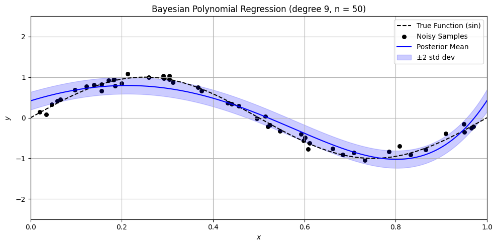
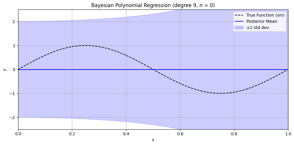
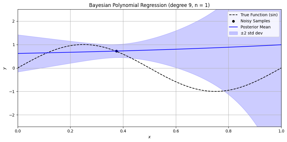
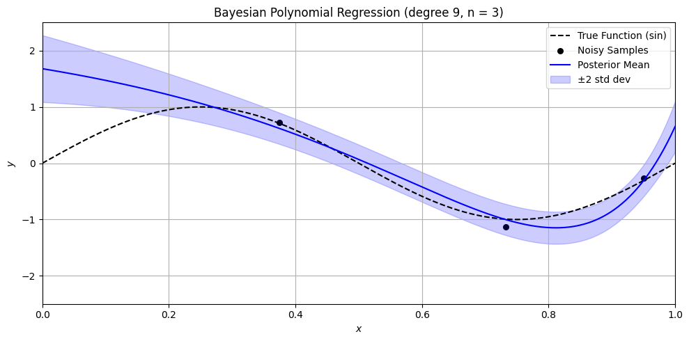
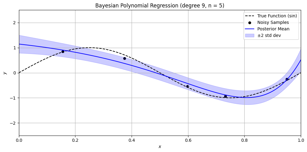
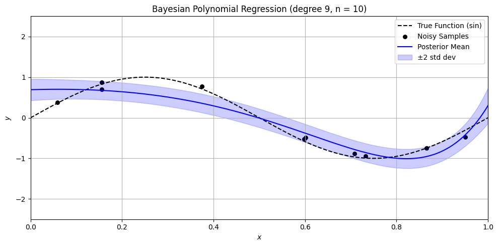
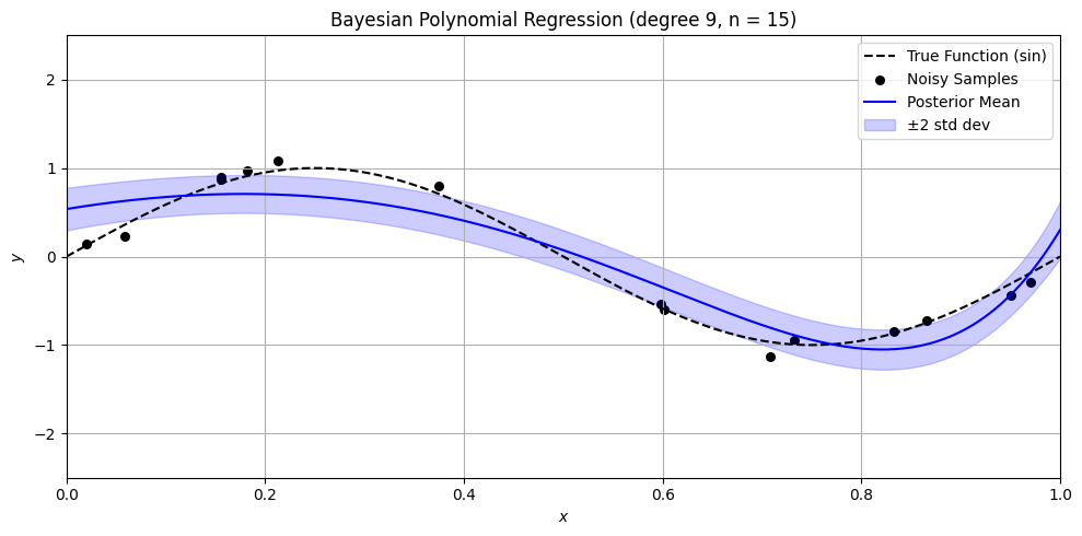
Bayesian Polynomial Regression Example#
Show code cell source
import numpy as np
import matplotlib.pyplot as plt
from sklearn.preprocessing import PolynomialFeatures

def sine_polynomial_bayes_posterior_viz_safe(n=15, degree=9, noise_std=0.1, alpha=1.0, seed=42):
    np.random.seed(seed)

    def true_func(x): return np.sin(2 * np.pi * x)

    # Generate full dataset
    Xr = np.random.rand(1000, 1)
    yr = np.random.randn(1000)

    # Generate test data
    X_test = np.linspace(0, 1, 500).reshape(-1, 1)
    y_true = true_func(X_test)

    # Polynomial features
    poly = PolynomialFeatures(degree, include_bias=True)
    X_test_poly = poly.fit_transform(X_test)

    d = X_test_poly.shape[1]

    # Prior on weights
    w0 = np.zeros(d)
    Lambda0 = alpha * np.eye(d)  # prior covariance
    Lambda0_inv = np.linalg.inv(Lambda0)

    if n > 0:
        X = np.sort(Xr[:n], axis=0)
        y = true_func(X).ravel() + yr[:n] * noise_std

        X_poly = poly.transform(X)

        # Posterior parameters
        sigma2 = noise_std ** 2
        precision_lik = (1 / sigma2) * (X_poly.T @ X_poly)
        precision_post = precision_lik + Lambda0_inv
        cov_post = np.linalg.inv(precision_post)
        mean_post = cov_post @ ((1 / sigma2) * X_poly.T @ y + Lambda0_inv @ w0)

    else:
        mean_post = w0
        cov_post = Lambda0

    # Posterior predictive mean and variance
    y_pred_mean = X_test_poly @ mean_post
    y_pred_var = np.sum(X_test_poly @ cov_post * X_test_poly, axis=1) + noise_std ** 2
    y_pred_std = np.sqrt(y_pred_var)

    # Plot with uncertainty bands
    plt.figure(figsize=(10, 5))
    plt.plot(X_test, y_true, 'k--', label='True Function (sin)')
    if n > 0:
        plt.scatter(X, y, color='black', s=30, label='Noisy Samples')
    plt.plot(X_test, y_pred_mean, 'b-', label='Posterior Mean')
    plt.fill_between(
        X_test.ravel(),
        y_pred_mean - 2 * y_pred_std,
        y_pred_mean + 2 * y_pred_std,
        color='blue',
        alpha=0.2,
        label='±2 std dev'
    )
    plt.title(f'Bayesian Polynomial Regression (degree {degree}, n = {n})')
    plt.xlabel('$x$')
    plt.ylabel('$y$')
    plt.ylim(-2.5, 2.5)
    plt.xlim(0, 1)
    plt.grid(True)
    plt.legend()
    plt.tight_layout()
    plt.show()

# Rerun with corrected safe handling for n = 0
n_values = [0, 1, 3, 5, 10, 15, 50]

for n in n_values:
    sine_polynomial_bayes_posterior_viz_safe(n=n, degree=9, alpha=1.0)
/var/folders/n7/1tlnr9g5403gj0lq5b926czm0000gn/T/ipykernel_8758/2531115809.py:47: RuntimeWarning: divide by zero encountered in matmul
  y_pred_mean = X_test_poly @ mean_post
/var/folders/n7/1tlnr9g5403gj0lq5b926czm0000gn/T/ipykernel_8758/2531115809.py:47: RuntimeWarning: overflow encountered in matmul
  y_pred_mean = X_test_poly @ mean_post
/var/folders/n7/1tlnr9g5403gj0lq5b926czm0000gn/T/ipykernel_8758/2531115809.py:47: RuntimeWarning: invalid value encountered in matmul
  y_pred_mean = X_test_poly @ mean_post
/var/folders/n7/1tlnr9g5403gj0lq5b926czm0000gn/T/ipykernel_8758/2531115809.py:48: RuntimeWarning: divide by zero encountered in matmul
  y_pred_var = np.sum(X_test_poly @ cov_post * X_test_poly, axis=1) + noise_std ** 2
/var/folders/n7/1tlnr9g5403gj0lq5b926czm0000gn/T/ipykernel_8758/2531115809.py:48: RuntimeWarning: overflow encountered in matmul
  y_pred_var = np.sum(X_test_poly @ cov_post * X_test_poly, axis=1) + noise_std ** 2
/var/folders/n7/1tlnr9g5403gj0lq5b926czm0000gn/T/ipykernel_8758/2531115809.py:48: RuntimeWarning: invalid value encountered in matmul
  y_pred_var = np.sum(X_test_poly @ cov_post * X_test_poly, axis=1) + noise_std ** 2
/var/folders/n7/1tlnr9g5403gj0lq5b926czm0000gn/T/ipykernel_8758/2531115809.py:37: RuntimeWarning: divide by zero encountered in matmul
  precision_lik = (1 / sigma2) * (X_poly.T @ X_poly)
/var/folders/n7/1tlnr9g5403gj0lq5b926czm0000gn/T/ipykernel_8758/2531115809.py:37: RuntimeWarning: overflow encountered in matmul
  precision_lik = (1 / sigma2) * (X_poly.T @ X_poly)
/var/folders/n7/1tlnr9g5403gj0lq5b926czm0000gn/T/ipykernel_8758/2531115809.py:37: RuntimeWarning: invalid value encountered in matmul
  precision_lik = (1 / sigma2) * (X_poly.T @ X_poly)
/var/folders/n7/1tlnr9g5403gj0lq5b926czm0000gn/T/ipykernel_8758/2531115809.py:47: RuntimeWarning: divide by zero encountered in matmul
  y_pred_mean = X_test_poly @ mean_post
/var/folders/n7/1tlnr9g5403gj0lq5b926czm0000gn/T/ipykernel_8758/2531115809.py:47: RuntimeWarning: overflow encountered in matmul
  y_pred_mean = X_test_poly @ mean_post
/var/folders/n7/1tlnr9g5403gj0lq5b926czm0000gn/T/ipykernel_8758/2531115809.py:47: RuntimeWarning: invalid value encountered in matmul
  y_pred_mean = X_test_poly @ mean_post
/var/folders/n7/1tlnr9g5403gj0lq5b926czm0000gn/T/ipykernel_8758/2531115809.py:48: RuntimeWarning: divide by zero encountered in matmul
  y_pred_var = np.sum(X_test_poly @ cov_post * X_test_poly, axis=1) + noise_std ** 2
/var/folders/n7/1tlnr9g5403gj0lq5b926czm0000gn/T/ipykernel_8758/2531115809.py:48: RuntimeWarning: overflow encountered in matmul
  y_pred_var = np.sum(X_test_poly @ cov_post * X_test_poly, axis=1) + noise_std ** 2
/var/folders/n7/1tlnr9g5403gj0lq5b926czm0000gn/T/ipykernel_8758/2531115809.py:48: RuntimeWarning: invalid value encountered in matmul
  y_pred_var = np.sum(X_test_poly @ cov_post * X_test_poly, axis=1) + noise_std ** 2