Moore-Penrose Pseudoinverse#
The Moore-Penrose pseudoinverse is a generalization of the matrix inverse that can be applied to non-square or singular matrices. It is denoted as \( \mathbf{A}^+ \) for a matrix \( \mathbf{A} \).
The pseudoinverse satisfies the following defining properties:
\( \mathbf{A} \mathbf{A}^+ \mathbf{A} = \mathbf{A} \)
\( \mathbf{A}^+ \mathbf{A} \mathbf{A}^+ = \mathbf{A}^+ \)
From these properties, we can derive the following additional properties:
\( (\mathbf{A} \mathbf{A}^+)^\top = \mathbf{A} \mathbf{A}^+ \)
\( (\mathbf{A}^+ \mathbf{A})^\top = \mathbf{A}^+ \mathbf{A} \)
Existence: The pseudoinverse exists for any matrix \( \mathbf{A} \).
Uniqueness: The pseudoinverse is unique.
Rank: The rank of \( \mathbf{A}^+ \) is equal to the rank of \( \mathbf{A} \).
Least Squares Solution: The pseudoinverse provides a least squares solution to the equation \( \mathbf{A}\mathbf{x} = \mathbf{b} \) when \( \mathbf{A} \) is not square or has no unique solution. The least squares solution is given by:
Geometric Interpretation: The pseudoinverse can be interpreted geometrically as the projection of a vector onto the column space of \( \mathbf{A} \). Computational Considerations: The computation of the pseudoinverse can be done efficiently using numerical methods, such as the SVD, especially for large matrices. Limitations: The pseudoinverse may not be suitable for all applications, especially when the matrix is ill-conditioned or has a high condition number.
The Pseudoinverse in Linear Regression#
In linear regression, we often encounter the problem of finding the best-fitting line (or hyperplane) through a set of data points. The Moore-Penrose pseudoinverse provides a tool for solving this problem, especially when the design matrix is not square or is singular.
1. Ordinary Least Squares (OLS) Problem#
Given data matrix \(\mathbf{X} \in \mathbb{R}^{n \times d}\), and target \(\mathbf{y} \in \mathbb{R}^{n}\), the OLS problem is:
Objective: Minimize the squared error between predictions and targets:
This is a quadratic problem with a closed-form solution if \( \mathbf{X}^\top \mathbf{X} \) is invertible:
OLS solution:
2. Observe: This Has the Structure of a Pseudoinverse#
We now define:
We claim that \( \mathbf{X}^+ \) is the Moore–Penrose pseudoinverse of \( \mathbf{X} \), and it satisfies the four defining properties — if \( \mathbf{X} \) has full column rank:
\( \mathbf{X}\mathbf{X}^+\mathbf{X} = \mathbf{X} \)
\( \mathbf{X}^+\mathbf{X}\mathbf{X}^+ = \mathbf{X}^+ \)
\( (\mathbf{X}\mathbf{X}^+)^\top = \mathbf{X}\mathbf{X}^+ \)
\( (\mathbf{X}^+\mathbf{X})^\top = \mathbf{X}^+\mathbf{X} \)
3. State the General Case: Unique Pseudoinverse Always Exists#
Regardless of whether \( \mathbf{X} \) has full column rank or not, there is a unique matrix \( \mathbf{X}^+ \in \mathbb{R}^{d \times n} \) satisfying all four Moore–Penrose conditions.
This is the Moore–Penrose pseudoinverse, and:
still gives the minimum-norm least squares solution, even if \(\mathbf{X}\) is not full rank.
4. Numerical Example Using NumPy’s pinv#
import numpy as np
import matplotlib.pyplot as plt
# Simulate linear data with collinearity
np.random.seed(1)
n, d = 100, 5
X = np.random.randn(n, d)
X[:, 3] = X[:, 1] + 0.01 * np.random.randn(n) # make column 3 nearly linearly dependent on column 1
beta_true = np.array([2.0, -1.0, 0.0, 0.5, 3.0])
y = X @ beta_true + np.random.randn(n) * 0.5
# Compute OLS via pseudoinverse
X_pinv = np.linalg.pinv(X) # Moore–Penrose pseudoinverse
beta_hat = X_pinv @ y
# Compare with np.linalg.lstsq (which uses SVD internally)
beta_lstsq, *_ = np.linalg.lstsq(X, y, rcond=None)
print("True coefficients: ", beta_true)
print("Estimated (pinv): ", beta_hat)
print("Estimated (lstsq): ", beta_lstsq)
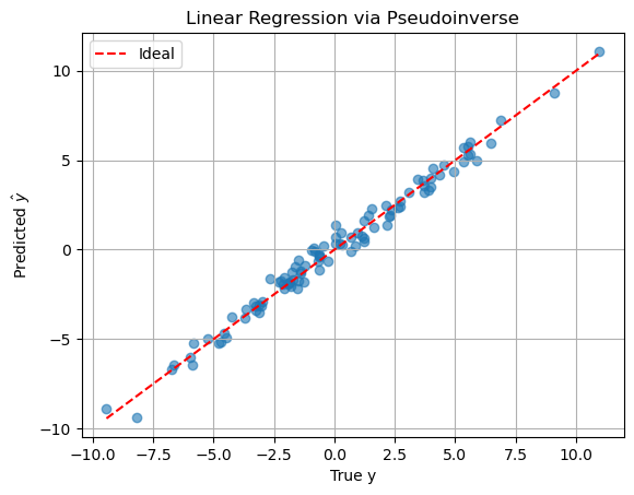
# Prediction
y_hat = X @ beta_hat
# Visualization
plt.scatter(y, y_hat, alpha=0.6)
plt.plot([y.min(), y.max()], [y.min(), y.max()], 'r--', label='Ideal')
plt.xlabel('True y')
plt.ylabel(r'Predicted $\hat{y}$')
plt.title('Linear Regression via Pseudoinverse')
plt.legend()
plt.grid(True)
plt.show()
True coefficients:      [ 2.  -1.   0.   0.5  3. ]
Estimated (pinv):       [ 1.94709549 -5.19769638 -0.04013046  4.70635095  2.98224449]
Estimated (lstsq):      [ 1.94709549 -5.19769638 -0.04013046  4.70635095  2.98224449]
The OLS formula is a special case of the pseudoinverse, valid under full column rank. The pseudoinverse is unique and always provides a least-squares solution.
Note that numpy.linalg.pinv computes the Moore–Penrose pseudoinverse using the Singular Value Decomposition (SVD). This method is both general and numerically stable, making it well-suited for pseudoinverse computation even when the matrix is not full rank.
How np.linalg.pinv Works Internally#
Suppose you have a matrix \(\mathbf{X} \in \mathbb{R}^{n \times d}\).
The pseudoinverse \(\mathbf{X}^+ \in \mathbb{R}^{d \times n}\) is computed as follows:
Step 1: Perform reduced SVD#
U, S, Vt = np.linalg.svd(X, full_matrices=False)
This gives:
Where:
\(\mathbf{U}_r \in \mathbb{R}^{n \times r}\), with orthonormal columns
\(\boldsymbol{\Sigma}_r \in \mathbb{R}^{r \times r}\), diagonal matrix with singular values \(\sigma_1, \dots, \sigma_r\)
\(\mathbf{V}_r \in \mathbb{R}^{d \times r}\), with orthonormal columns
\(r = \text{rank}(\mathbf{X})\)
Step 2: Invert the Non-Zero Singular Values#
You construct the diagonal matrix \(\boldsymbol{\Sigma}_r^+ \in \mathbb{R}^{r \times r}\) as:
This step thresholds small singular values using the rcond parameter (default: machine epsilon).
Step 3: Recompose the Pseudoinverse#
The pseudoinverse is then:
In code:
def pinv_manual(X, rcond=1e-15):
    U, S, Vt = np.linalg.svd(X, full_matrices=False)
    S_inv = np.array([1/s if s > rcond * S[0] else 0 for s in S])
    return Vt.T @ np.diag(S_inv) @ U.T
✅ Advantages of SVD-Based Pseudoinverse#
Numerically stable: even if \(\mathbf{X}^\top \mathbf{X}\) is ill-conditioned
General: works for rank-deficient or rectangular matrices
Gives minimum-norm solution to \(\mathbf{X}\boldsymbol{\beta} = \mathbf{y}\)
🧪 Check with NumPy#
You can verify this approach:
X = np.random.randn(5, 3)
X_pinv_np = np.linalg.pinv(X)
X_pinv_manual = pinv_manual(X)

np.allclose(X_pinv_np, X_pinv_manual)  # Should be True
True