Newton’s Method#
Newton’s method is a powerful optimization algorithm that leverages both the gradient and the Hessian (second derivative) of a function to find its local minima or maxima. Unlike first-order methods such as gradient descent, which use only slope information, Newton’s method uses curvature information to make more informed and often much faster progress toward a solution.
In this section, we’ll introduce the intuition behind Newton’s method, derive its update rule from the second-order Taylor expansion, and discuss its strengths and limitations. We’ll also see how Newton’s method can be improved in practice, for example by incorporating line search techniques to ensure robust convergence.
Many functions are challenging to minimize directly, but quadratic functions have a simple, closed-form solution for their minimum. Newton’s method leverages this by constructing a local quadratic approximation of the objective function at the current point using the second-order Taylor expansion. Instead of minimizing the original (potentially complicated) function, Newton’s method minimizes this quadratic surrogate at each step. Although the minimum of the quadratic approximation will generally not be the true minimum of the original function, iteratively updating the approximation and repeating the process can rapidly lead us toward a local minimum.
Motivation from Second-Order Taylor Expansion#
Recall the second-order Taylor expansion of a function \(f: \mathbb{R}^d \to \mathbb{R}\) around a point \(\mathbf{x}_0\):
We now minimize this quadratic approximation with respect to \(\mathbf{x}\). The minimum occurs where the gradient vanishes:
Solving for \(\mathbf{x}\), we get the Newton update rule:
Newton’s Method: Iterative Algorithm#
Given an initial guess \(\mathbf{x}_0\), we repeat:
until convergence.
Note, that we assume that the Hessian is invertible. In practice, we can avoid computing the inverse of the Hessian by solving the linear system \(\nabla^2 f(\mathbf{x}_k) \mathbf{d}_k = -\nabla f(\mathbf{x}_k)\) for the Newton step \(\mathbf{d}_k\).
Unlike gradient descent, which moves in the direction of steepest descent, Newton’s method uses second-order curvature information to take a more direct path toward the minimum.
Let’s implement a class for Newton’s method:
class Newton:
    def __init__(self, f, grad_f, hess_f, x0, tol=1e-6, max_iter=20):
        self.f = f
        self.grad_f = grad_f
        self.hess_f = hess_f
        self.x0 = x0
        self.tol = tol
        self.max_iter = max_iter
        self.path = []

    def run(self):
        x = self.x0
        self.path.append(x)
        for _ in range(self.max_iter):
            grad = self.grad_f(x)
            hess = self.hess_f(x)
            # Compute the Newton step by solving the linear system
            d = np.linalg.solve(hess, grad)
            x = x - d # Update the iterate
            if np.linalg.norm(grad) < self.tol:
                break
            self.path.append(x)
        return x, np.array(self.path)
Let’s test it on a simple function \(f(x) = e^{x} + x^2\) and plot the path taken by Newton’s method:
Show code cell source
import numpy as np
import matplotlib.pyplot as plt

def f(x):
    return np.exp(x) + x**2

def grad_f(x):
    return np.exp(x) + 2 * x

def hess_f(x):
    return np.exp(x) + 2 * np.eye(len(x))

newton = Newton(f, grad_f, hess_f, x0=np.array([1.0]))
x_star, path = newton.run()

x_vals = np.linspace(-1, 1.05, 100)
y_vals = f(x_vals)

plt.plot(x_vals, y_vals)
plt.plot(newton.path, [f(x) for x in newton.path], 'ro-')
plt.xlim(-1, 1.05)
plt.show()
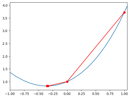
We see that Newton’s method rapidly converges to the minimum.
Convergence of Newton’s Method#
It turns out that convergence of Newton’s method is not guaranteed for all functions. We will see that for convex functions, Newton’s method converges quadratically to the minimum. However, for non-convex functions, the convergence is only guaranteed locally near a point where the Hessian is positive definite.
In fact, if the Hessian is not positive definite, the update may not be a descent direction.
To see this, let’s consider the following non-convex function:
Let’s plot the function and the path taken by Newton’s method, starting from the point \((0, -1)\):
Show code cell source
from mpl_toolkits.mplot3d import Axes3D

def f(x):
    return x[0]**2 - x[1]**2

def grad_f(x):
    return np.array([2 * x[0], -2 * x[1]])

def hess_f(x):
    return np.array([[2, 0], [0, -2]])

newton = Newton(f, grad_f, hess_f, x0=np.array([0., -1.0]))
newton.run()

x_vals = np.linspace(-1.1, 1.1, 100)
y_vals = np.linspace(-1.1, 1.1, 100)
X, Y = np.meshgrid(x_vals, y_vals)
Z = f(np.array([X, Y]))

fig = plt.figure()
ax = fig.add_subplot(111, projection='3d')
ax.plot_surface(X, Y, Z, cmap='viridis', alpha=0.6)

# Plot the path taken by Newton's method
for x in newton.path:
    ax.scatter(x[0], x[1], f(x), color='r', s=50)

ax.set_xlabel('X')
ax.set_ylabel('Y')
ax.set_zlabel('f(x, y)')

plt.show()
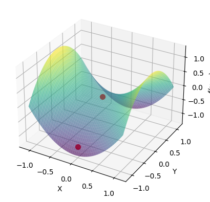
We see that Newton’s method does not converge to a minimum but rather to the saddle point at \((0, 0)\). In fact, we observe that the function increases in the direction of the Newton step.
Let’s look at another non-convex example:
The function has a single minimum close to the initial point \((1.5, 1.5)\).
Show code cell source
import numpy as np
import matplotlib.pyplot as plt
from mpl_toolkits.mplot3d import Axes3D

# Define the function, gradient, and Hessian
def f(x):
    return np.log(1 + np.sum(x**2))

def grad_f(x):
    return 2 * x / (1 + np.sum(x**2))

def hess_f(x):
    r2 = np.sum(x**2)
    I = np.eye(len(x))
    outer = np.outer(x, x)
    return (2 / (1 + r2)) * I - (4 / (1 + r2)**2) * outer

# Run the method
x0 = np.array([1.5, 1.5])
newton = Newton(f, grad_f, hess_f, x0)
x_star, path = newton.run()

# Create grid for visualization
x_vals = np.linspace(-2, 8, 100)
y_vals = np.linspace(-2, 8, 100)
X, Y = np.meshgrid(x_vals, y_vals)
Z = np.log(1 + X**2 + Y**2)

# Compute the Taylor expansion around x0
f0 = f(x0)
grad0 = grad_f(x0)
hess0 = hess_f(x0)
# print(hess0)
eigvals, eigvecs = np.linalg.eigh(hess0)

# Taylor expansion: f(x) ≈ f(x0) + grad_f(x0) * (x - x0) + 0.5 * (x - x0)^T * hess_f(x0) * (x - x0)
def taylor_approx(x, y):
    xy = np.array([x, y])
    delta = xy - x0
    return f0 + grad0 @ delta + 0.5 * delta @ hess0 @ delta

# Compute the Taylor approximation surface
Z_taylor = np.array([[taylor_approx(x, y) for x, y in zip(x_row, y_row)] for x_row, y_row in zip(X, Y)])

# Plot
fig = plt.figure(figsize=(10, 6))
ax = fig.add_subplot(111, projection='3d')
ax.plot_surface(X, Y, Z, cmap='viridis', alpha=0.6) # , label='Original Function'
# ax.plot_surface(X, Y, Z_taylor, cmap='autumn', alpha=0.4, label='Taylor Expansion')

# Overlay path
ax.plot(path[:3, 0], path[:3, 1], [f(p) for p in path[:3,:]], color='red', marker='o', label="Newton steps")
ax.scatter(*x0, f(x0), color='blue', label=r'Initial point $\mathbf{x}_0$', s=60)
# ax.scatter(*path[-1], f(path[-1]), color='green', label='Final point', s=60)

ax.set_title(r"Newton's Method on $f(x, y) = \log(1 + x^2 + y^2)$")
ax.set_xlabel("x")
ax.set_ylabel("y")
ax.legend()
plt.tight_layout()
plt.show()
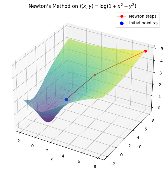
We observe that the Newton step is not a descent direction at the initial point, and Newton’s method diverges. If we look at the Hessian at the initial point, we see that it is not positive definite:
Show code cell source
print(r"Hessian at the initial point (1.5, 1.5):")
print(hess0)
print("Eigenvalues: ", eigvals)
# print(eigvals)
# print("Eigenvectors:")
# print(eigvecs)
Hessian at the initial point (1.5, 1.5):
[[ 0.0661157  -0.29752066]
 [-0.29752066  0.0661157 ]]
Eigenvalues:  [-0.23140496  0.36363636]
To better understand why Newton’s method diverges and how this relates to the eigenvalues of the Hessian, let’s look at the directional derivative of \(f\) in the direction of the Newton step.
To do so, let’s introduce a one-dimensional function \(g(t) = f(x_k + t \left[\nabla^2 f(\mathbf{x}_k)\right]^{-1} \nabla f(\mathbf{x}_k))\).
Then the first derivative of \(g(t)\) is equal to the directional derivative of \(f\) in the direction of the Newton step:
To see, what happens if the Hessian is not positive definite as in the example above, let’s replace it with its eigendecomposition:
For \(t = 0\), we have:
We can rewrite the derivative as a sum of the directional derivatives in the directions of the eigenvectors \(q_i\) of the Hessian:
If the Hessian is positive definite, then all of the terms are positive and the sum is guaranteed to be positive. However, if the Hessian is not positive definite, then not all eigenvalues \(\lambda_i\) are positive. Thus, for non-convex functions the sum is not guaranteed to be positive. In that case, the Newton step is not guaranteed to be a descent direction, and may even be a direction of ascent as in the example above.
Convergence for Convex Functions#
As we have just shown, for striclty convex functions, where the Hessian is guaranteed to be positive definite everywhere, the Newton step is a descent direction. Additionally, we can show that Newton’s method is guaranteed to get to a minimum rapidly.
Theorem (Quadratic Convergence for Convex Functions)
Let \(f(x)\) be a convex function. Then
where \(L\) is the Lipschitz constant of the Hessian.
This means that the error between \(x_k\) and the optimal solution \(x^*\) decreases quadratically.
Proof. Let \(f: \mathbb{R}^n \to \mathbb{R}\) be a twice continuously differentiable convex function, and suppose the Hessian \(\nabla^2 f(x)\) is Lipschitz continuous with constant \(L\) in a neighborhood of the minimizer \(x^*\).
Assume also that \(\nabla^2 f(x^*)\) is positive definite (i.e., \(f\) is strictly convex).
Let \(x_k\) be the current iterate, and define the Newton step:
Let \(e_k = x_k - x^*\).
By Taylor’s theorem,
where the remainder \(r_k\) satisfies
The Newton update gives:
If \(x_k\) is close to \(x^*\), then \(\nabla^2 f(x_k) \approx \nabla^2 f(x^*)\), so the first term is small (of order \(\|e_k\|^2\)), and the second term is also of order \(\|e_k\|^2\) due to the bound on \(r_k\).
Therefore, there exists a constant \(C > 0\) such that
for all \(x_k\) sufficiently close to \(x^*\). This is quadratic convergence.
Finally, since \(f\) is convex and the Hessian is Lipschitz, we also have
as stated.
Conclusion: Under the stated conditions, Newton’s method converges quadratically to the minimizer \(x^*\), and the function value error decreases at least as fast as \(\|x_k - x^*\|^2\).
Convergence for Non-convex functions#
For non-convex functions, the convergence is only guaranteed locally near a point where the Hessian is positive definite.
Theorem (Local Convergence for Non-convex Functions)
Let \(f(x)\) be a twice continuously differentiable function, and assume that the Hessian \(\nabla^2 f(x)\) is Lipschitz continuous with constant \(L\) in a neighborhood of a local minimum \(x^*\).
If \(x_k\) is sufficiently close to \(x^*\) and the Hessian is positive definite at \(x^*\), then Newton’s method exhibits quadratic convergence.
Specifically, the following inequality holds:
This result is particularly relevant for convex functions, where global convergence can be more readily assured. However, for non-convex functions, the convergence is only guaranteed locally near a point where the Hessian is positive definite.
Why Newton’s Method Alone Can Fail#
The Newton update:
assumes that the Hessian is positive definite, which ensures a descent direction and local convexity. But in practice:
The Hessian may be indefinite (especially far from the minimum).
The step \(\Delta \mathbf{x}\) can be too large, causing divergence.
Line Search to the Rescue#
To improve robustness, we combine Newton’s direction with a line search:
Here, \(\eta_k\) is chosen using a backtracking line search, typically satisfying the Armijo condition (just like in gradient descent).
Newton’s Method with Line Search: Pseudocode#
Compute Newton direction: \(\mathbf{d}_k = -[\nabla^2 f(\mathbf{x}_k)]^{-1} \nabla f(\mathbf{x}_k)\)
Perform line search: Find \(\eta_k \in (0, 1]\) such that
\[ f(\mathbf{x}_k + \eta_k \mathbf{d}_k) \leq f(\mathbf{x}_k) + c_1 \eta_k \nabla f(\mathbf{x}_k)^\top \mathbf{d}_k \]Update: \(\mathbf{x}_{k+1} = \mathbf{x}_k + \eta_k \mathbf{d}_k\)
Handles indefinite or ill-conditioned Hessians
Prevents overshooting
Preserves fast convergence near the minimum
Makes Newton’s method practical for real optimization problems
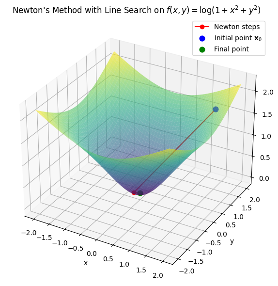
Newton’s Method with Armijo Backtracking#
Here’s a modified version of our Newton’s method implementation, now with several tricks added to keep Newton’s method fast and stable.
Armijo backtracking line search ensures each step decreases the objective. It can reduce the step size in cases where full Newton steps are too aggressive.
Spectral decomposition of the Hessian allows us to detect cases where the Hessian is ill-conditioned and modify the eigenvalues to enforce positive definiteness.
class NewtonWithBacktracking:
    def __init__(self, f, grad_f, hess_f, x0, tol=1e-6, max_iter=20, eps=1e-8):
        self.f = f
        self.grad_f = grad_f
        self.hess_f = hess_f
        self.x0 = x0
        self.tol = tol
        self.max_iter = max_iter
        self.eps = eps
        self.path = []
        self.etas = []

    def armijo_backtracking(self, x, d, alpha=1.0, beta=0.5, c1=1e-4):
        f_x = self.f(x)
        grad_dot_d = self.grad_f(x).dot(d)
        while self.f(x + alpha * d) > f_x + c1 * alpha * grad_dot_d:
            alpha *= beta
        return alpha

    def run(self):
        x = self.x0.copy()
        self.path.append(x.copy())

        for _ in range(self.max_iter):
            grad = self.grad_f(x)
            H = self.hess_f(x)
            eigvals, eigvecs = np.linalg.eigh(H)
            eigvals[eigvals < self.eps] = self.eps  # Ensure positive definiteness
            d = - eigvecs @ (1.0/eigvals * (eigvecs.T @ grad))  # Compute the Newton step
            eta = self.armijo_backtracking(x, d)
            x = x + eta * d
            self.path.append(x.copy())
            self.etas.append(eta)

        return x, np.array(self.path), self.etas
Show code cell source
import numpy as np
import matplotlib.pyplot as plt
from mpl_toolkits.mplot3d import Axes3D
# Define the function, gradient, and Hessian
def f(x):
    return np.log(1 + np.sum(x**2))

def grad_f(x):
    return 2 * x / (1 + np.sum(x**2))

def hess_f(x):
    r2 = np.sum(x**2)
    I = np.eye(len(x))
    outer = np.outer(x, x)
    return (2 / (1 + r2)) * I - (4 / (1 + r2)**2) * outer

# Run the method
x0 = np.array([1.5, 1.5])
newton = NewtonWithBacktracking(f, grad_f, hess_f, x0)
x_star, path, etas = newton.run()

# Create grid for visualization
x_vals = np.linspace(-2, 2, 100)
y_vals = np.linspace(-2, 2, 100)
X, Y = np.meshgrid(x_vals, y_vals)
Z = np.log(1 + X**2 + Y**2)

# Plot
fig = plt.figure(figsize=(10, 6))
ax = fig.add_subplot(111, projection='3d')
ax.plot_surface(X, Y, Z, cmap='viridis', alpha=0.6)

# Overlay path
ax.plot(path[:, 0], path[:, 1], [f(p) for p in path], color='red', marker='o', label="Newton steps")
ax.scatter(*x0, f(x0), color='blue', label=r'Initial point $\mathbf{x}_0$', s=60)
ax.scatter(*path[-1], f(path[-1]), color='green', label='Final point', s=60)

ax.set_title(r"Newton's Method with Line Search on $f(x, y) = \log(1 + x^2 + y^2)$")
ax.set_xlabel("x")
ax.set_ylabel("y")
ax.legend()
plt.tight_layout()
plt.show()