Estimation of Parameters

Estimation of Parameters#

Now we get into some basic topics from statistics. We make some assumptions about our problem by prescribing a parametric model (e.g. a distribution that describes how the data were generated), then we fit the parameters of the model to the data. How do we choose the values of the parameters?

Maximum likelihood estimation#

A common way to fit parameters is maximum likelihood estimation (MLE). The basic principle of MLE is to choose values that “explain” the data best by maximizing the probability/density of the data we’ve seen as a function of the parameters. Suppose we have random variables \(X_1, \dots, X_n\) and corresponding observations \(x_1, \dots, x_n\). Then

\[ \hat{\mathbf{\theta}}_\text{mle} = \operatorname{argmax}_\mathbf{\theta} \mathcal{L}(\mathbf{\theta}) \]

where \(\mathcal{L}\) is the likelihood function

\[ \mathcal{L}(\mathbf{\theta}) = p(x_1, \dots, x_n; \mathbf{\theta}) \]

Often, we assume that \(X_1, \dots, X_n\) are i.i.d. Then we can write

\[p(x_1, \dots, x_n; \theta) = \prod_{i=1}^n p(x_i; \mathbf{\theta})\]

At this point, it is usually convenient to take logs, giving rise to the log-likelihood

\[\log\mathcal{L}(\mathbf{\theta}) = \sum_{i=1}^n \log p(x_i; \mathbf{\theta})\]

This is a valid operation because the probabilities/densities are assumed to be positive, and since log is a monotonically increasing function, it preserves ordering. In other words, any maximizer of \(\log\mathcal{L}\) will also maximize \(\mathcal{L}\).

For some distributions, it is possible to analytically solve for the maximum likelihood estimator. If \(\log\mathcal{L}\) is differentiable, setting the derivatives to zero and trying to solve for \(\mathbf{\theta}\) is a good place to start.

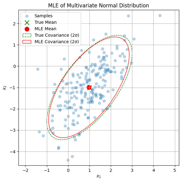
Maximum Likelihood Estimation for the Multivariate Normal#

Suppose we observe data points \(\mathbf{x}_1, \dots, \mathbf{x}_n \in \mathbb{R}^d\) assumed to be i.i.d. samples from a multivariate normal distribution with unknown parameters:

\[ \mathbf{x}_i \sim \mathcal{N}(\boldsymbol{\mu}, \boldsymbol{\Sigma}) \]

We want to estimate \(\boldsymbol{\mu} \in \mathbb{R}^d\) and \(\boldsymbol{\Sigma} \in \mathbb{R}^{d \times d}\), where \(\boldsymbol{\Sigma}\) is symmetric and positive definite.

Step 1: Write the Likelihood#

The density of the multivariate normal is:

\[ p(\mathbf{x}_i; \boldsymbol{\mu}, \boldsymbol{\Sigma}) = \frac{1}{(2\pi)^{d/2} |\boldsymbol{\Sigma}|^{1/2}} \exp\left( -\frac{1}{2} (\mathbf{x}_i - \boldsymbol{\mu})^\top \boldsymbol{\Sigma}^{-1} (\mathbf{x}_i - \boldsymbol{\mu}) \right) \]

Since the samples are i.i.d., the joint likelihood is:

\[ \mathcal{L}(\boldsymbol{\mu}, \boldsymbol{\Sigma}) = \prod_{i=1}^n p(\mathbf{x}_i; \boldsymbol{\mu}, \boldsymbol{\Sigma}) \]

Step 2: Take the Log-Likelihood#

Take logarithms to get a sum:

\[\begin{split} \begin{aligned} \log \mathcal{L}(\boldsymbol{\mu}, \boldsymbol{\Sigma}) &= \sum_{i=1}^n \log p(\mathbf{x}_i; \boldsymbol{\mu}, \boldsymbol{\Sigma}) \\ &= \sum_{i=1}^n \left[ -\frac{d}{2} \log(2\pi) - \frac{1}{2} \log |\boldsymbol{\Sigma}| - \frac{1}{2} (\mathbf{x}_i - \boldsymbol{\mu})^\top \boldsymbol{\Sigma}^{-1} (\mathbf{x}_i - \boldsymbol{\mu}) \right] \\ &= -\frac{nd}{2} \log(2\pi) - \frac{n}{2} \log |\boldsymbol{\Sigma}| - \frac{1}{2} \sum_{i=1}^n (\mathbf{x}_i - \boldsymbol{\mu})^\top \boldsymbol{\Sigma}^{-1} (\mathbf{x}_i - \boldsymbol{\mu}) \end{aligned} \end{split}\]

Only the last two terms depend on the parameters, so we optimize:

\[ \ell(\boldsymbol{\mu}, \boldsymbol{\Sigma}) := - \frac{n}{2} \log |\boldsymbol{\Sigma}| - \frac{1}{2} \sum_{i=1}^n (\mathbf{x}_i - \boldsymbol{\mu})^\top \boldsymbol{\Sigma}^{-1} (\mathbf{x}_i - \boldsymbol{\mu}) \]

Step 3a: Maximize with Respect to \(\boldsymbol{\mu}\)#

We take the gradient with respect to \(\boldsymbol{\mu}\):

\[\begin{split} \begin{aligned} \frac{\partial \ell}{\partial \boldsymbol{\mu}} &= \frac{1}{2} \sum_{i=1}^n \left[ \frac{\partial}{\partial \boldsymbol{\mu}} \left( - (\mathbf{x}_i - \boldsymbol{\mu})^\top \boldsymbol{\Sigma}^{-1} (\mathbf{x}_i - \boldsymbol{\mu}) \right) \right] \\ &= \sum_{i=1}^n \boldsymbol{\Sigma}^{-1} (\mathbf{x}_i - \boldsymbol{\mu}) \end{aligned} \end{split}\]

Set the derivative to zero:

\[ \sum_{i=1}^n \boldsymbol{\Sigma}^{-1} (\mathbf{x}_i - \boldsymbol{\mu}) = 0 \quad \Rightarrow \quad \sum_{i=1}^n (\mathbf{x}_i - \boldsymbol{\mu}) = 0 \quad \Rightarrow \quad n \boldsymbol{\mu} = \sum_{i=1}^n \mathbf{x}_i \]

So the MLE for the mean is:

\[ \hat{\boldsymbol{\mu}}_{\text{MLE}} = \frac{1}{n} \sum_{i=1}^n \mathbf{x}_i \]

Step 3b: Maximize with Respect to \(\boldsymbol{\Sigma}\)#

Substitute \(\hat{\boldsymbol{\mu}}\) into the log-likelihood:

Define the centered data:

\[ \mathbf{x}_i^c := \mathbf{x}_i - \hat{\boldsymbol{\mu}} \]

Then the negative log-likelihood becomes:

\[ \ell(\boldsymbol{\Sigma}) = -\frac{n}{2} \log |\boldsymbol{\Sigma}| - \frac{1}{2} \sum_{i=1}^n (\mathbf{x}_i^c)^\top \boldsymbol{\Sigma}^{-1} \mathbf{x}_i^c \]

We define the scatter matrix:

\[ \mathbf{S} = \sum_{i=1}^n \mathbf{x}_i^c (\mathbf{x}_i^c)^\top \]

Then:

\[ \ell(\boldsymbol{\Sigma}) = -\frac{n}{2} \log |\boldsymbol{\Sigma}| - \frac{1}{2} \operatorname{Tr}(\boldsymbol{\Sigma}^{-1} \mathbf{S}) \]

Take the derivative with respect to \(\boldsymbol{\Sigma}^{-1}\) (using matrix calculus):

\[ \frac{\partial \ell}{\partial \boldsymbol{\Sigma}^{-1}} = \frac{n}{2} \boldsymbol{\Sigma} - \frac{1}{2} \mathbf{S} \]

Set to zero:

\[ \Rightarrow\quad \frac{n}{2} \boldsymbol{\Sigma} = \frac{1}{2} \mathbf{S} \quad \Rightarrow \quad \hat{\boldsymbol{\Sigma}}_{\text{MLE}} = \frac{1}{n} \mathbf{S} = \frac{1}{n} \sum_{i=1}^n (\mathbf{x}_i - \hat{\boldsymbol{\mu}})(\mathbf{x}_i - \hat{\boldsymbol{\mu}})^\top \]

Summary#

The MLE for multivariate normal distribution yields:

Mean vector:

\[ \hat{\boldsymbol{\mu}} = \frac{1}{n} \sum_{i=1}^n \mathbf{x}_i \]
Covariance matrix:

\[ \hat{\boldsymbol{\Sigma}} = \frac{1}{n} \sum_{i=1}^n (\mathbf{x}_i - \hat{\boldsymbol{\mu}})(\mathbf{x}_i - \hat{\boldsymbol{\mu}})^\top \]

This is the sample mean and the (biased) sample covariance (with denominator \(n\)).

Show code cell source Hide code cell source

# Re-import required libraries after kernel reset
import numpy as np
import matplotlib.pyplot as plt
from matplotlib.patches import Ellipse
from scipy.stats import multivariate_normal

def plot_cov_ellipse(mean, cov, ax, n_std=2.0, facecolor='none', edgecolor='black', linestyle='-', label=None):
    """Add a 2D covariance ellipse to an existing plot."""
    vals, vecs = np.linalg.eigh(cov)
    order = vals.argsort()[::-1]
    vals, vecs = vals[order], vecs[:, order]
    theta = np.degrees(np.arctan2(*vecs[:, 0][::-1]))

    width, height = 2 * n_std * np.sqrt(vals)
    ellipse = Ellipse(xy=mean, width=width, height=height, angle=theta,
                      facecolor=facecolor, edgecolor=edgecolor, linestyle=linestyle, label=label)
    ax.add_patch(ellipse)

def mle_multivariate_normal_demo(n=200, d=2, seed=42):
    np.random.seed(seed)

    # True parameters
    mu_true = np.array([1.0, -1.0])
    Sigma_true = np.array([[1.0, 0.8],
                           [0.8, 1.5]])

    # Generate data
    X = np.random.multivariate_normal(mu_true, Sigma_true, size=n)

    # MLE estimates
    mu_mle = np.mean(X, axis=0)
    Sigma_mle = np.cov(X.T, bias=True)  # bias=True uses 1/n

    print("True mean:", mu_true)
    print("MLE mean :", mu_mle)
    print("True covariance:\n", Sigma_true)
    print("MLE covariance:\n", Sigma_mle)

    # Plot
    fig, ax = plt.subplots(figsize=(6, 6))
    ax.scatter(X[:, 0], X[:, 1], alpha=0.3, label='Samples')
    ax.scatter(*mu_true, c='green', marker='x', s=100, label='True Mean')
    ax.scatter(*mu_mle, c='red', marker='o', s=100, label='MLE Mean')

    # Add 2-sigma ellipses
    plot_cov_ellipse(mu_true, Sigma_true, ax, n_std=2.0, edgecolor='green', linestyle='--', label='True Covariance (2σ)')
    plot_cov_ellipse(mu_mle, Sigma_mle, ax, n_std=2.0, edgecolor='red', linestyle='-', label='MLE Covariance (2σ)')

    ax.set_title("MLE of Multivariate Normal Distribution")
    ax.set_xlabel("$x_1$")
    ax.set_ylabel("$x_2$")
    ax.grid(True)
    ax.axis('equal')
    ax.legend()
    plt.tight_layout()
    plt.show()

# Run the demo
mle_multivariate_normal_demo()

True mean: [ 1. -1.]
MLE mean : [ 0.9745329  -0.99265192]
True covariance:
 [[1.  0.8]
 [0.8 1.5]]
MLE covariance:
 [[0.89347252 0.72037511]
 [0.72037511 1.39413223]]

../_images/0655070ee13c6770048babea2229b53342cf434b34229000f084d0c1f5881d59.png

Maximum Likelihood Estimation for Linear Regression#

The likelihood is:

\[ p(\mathbf{y} \mid \mathbf{w}) = \prod_{i=1}^n \mathcal{N}(y_i \mid \mathbf{x}_i^\top \mathbf{w}, \sigma^2) \]

The log-likelihood is:

\[ \log p(\mathbf{y} \mid \mathbf{w}) = -\frac{1}{2\sigma^2} \|\mathbf{y} - \mathbf{Xw}\|^2 + \text{const} \]

So we observe that maximizing the log-likelihood is equivalent to minimizing the squared error.

\[ \hat{\mathbf{w}}_{\text{MLE}} = \operatorname{argmin}_\mathbf{w} \|\mathbf{y} - \mathbf{Xw}\|^2 \]

So the MLE for the linear regression model is identical to the OLS estimator:

\[ \hat{\mathbf{w}}_{\text{MLE}} = (\mathbf{X}^\top \mathbf{X})^{-1} \mathbf{X}^\top \mathbf{y} \]

Based on the estimator for the weights, we can also derive the estimator for the variance. In order to do this, we need to know the gradient of the log-likelihood with respect to the noise variance.

\[ \frac{\partial \log p(\mathbf{y} \mid \mathbf{w})}{\partial \sigma^2} = -\frac{n}{2\sigma^2} + \frac{1}{2\sigma^4} \|\mathbf{y} - \mathbf{Xw}\|^2 \]

Setting the gradient to zero, we get:

\[ \frac{\partial \log p(\mathbf{y} \mid \mathbf{w})}{\partial \sigma^2} = -\frac{n}{2\sigma^2} + \frac{1}{2\sigma^4} \|\mathbf{y} - \mathbf{Xw}\|^2 = 0 \]

Solving for \(\sigma^2\), we get:

\[ \hat{\sigma}^2 = \frac{1}{n} \|\mathbf{y} - \mathbf{X}\hat{\mathbf{w}}\|^2 \]

Limitations of MLE in Linear Regression#

While maximum likelihood estimation (MLE) is appealing for its simplicity and optimality under large samples, it has important drawbacks — especially in the context of linear regression with limited data or high-dimensional features.

Example: \(n = d\)#

Consider a linear regression model:

\[ y_i = \mathbf{x}_i^\top \mathbf{w} + \varepsilon_i, \quad \varepsilon_i \sim \mathcal{N}(0, \sigma^2) \]

Suppose the number of observations \(n\) is equal to the number of features \(d\). Then the design matrix \(\mathbf{X} \in \mathbb{R}^{n \times d}\) is square, and the MLE is:

\[ \hat{\mathbf{w}}_{\text{MLE}} = (\mathbf{X}^\top \mathbf{X})^{-1} \mathbf{X}^\top \mathbf{y} \]

In this case, \(\mathbf{X}^\top \mathbf{X}\) is invertible (with probability 1 if \(\mathbf{X}\) is random), and the MLE will perfectly interpolate the data — giving zero training error:

\[ \mathbf{y} = \mathbf{X} \hat{\mathbf{w}}_{\text{MLE}} \quad \Rightarrow \quad \|\mathbf{y} - \mathbf{X} \hat{\mathbf{w}}_{\text{MLE}}\|^2 = 0 \]

Problem: Overfitting and Variance Underestimation#

The MLE predicts with zero error on training data, but may generalize poorly to new inputs.
The estimated variance becomes:

\[ \hat{\sigma}^2 = \frac{1}{n} \|\mathbf{y} - \mathbf{X} \hat{\mathbf{w}}\|^2 = 0 \]

even though we know the data were generated with non-zero noise (\(\sigma^2 > 0\))!

❗ MLE underestimates the variance and is overconfident — especially when \(n\) is small or close to \(d\).

Key Insight#

Small sample sizes lead to overfitting with MLE.
Estimated noise variance can be zero when the model interpolates the data.
We need a way to regularize the parameter estimates and account for uncertainty.

Bayesian Fix: Maximum a Posteriori Estimation#

Maximum a posteriori estimation (MAP) allows us to introduce prior beliefs about the parameters to avoid this degeneracy.

For the multivariate normal, using an appropriate prior distribution allows us to derive a MAP estimate that:
- Shrinks the sample covariance toward a prior value
- Stays well-defined even when \(n = 1\)
- Regularizes estimates in low-data regimes

MAP estimation thus balances data and prior — resulting in more robust parameter estimates when the data are scarce.

In this technique we assume that the parameters are a random variable, and we specify a prior distribution \(p(\mathbf{\theta})\).

Then we can employ Bayes’ rule to compute the posterior distribution of the parameters given the observed data:

\[p(\mathbf{\theta} | x_1, \dots, x_n) \propto p(\mathbf{\theta})p(x_1, \dots, x_n | \mathbf{\theta})\]

Computing the normalizing constant is often intractable, because it involves integrating over the parameter space, which may be very high-dimensional. Fortunately, if we just want the MAP estimate, we don’t care about the normalizing constant! It does not affect which values of \(\mathbf{\theta}\) maximize the posterior.

So we have

\[\hat{\mathbf{\theta}}_\text{map} = \operatorname{argmax}_\mathbf{\theta} p(\mathbf{\theta})p(x_1, \dots, x_n | \mathbf{\theta})\]

Again, if we assume the observations are i.i.d., then we can express this in the equivalent, and possibly friendlier, form

\[\hat{\mathbf{\theta}}_\text{map} = \operatorname{argmax}_\mathbf{\theta} \left(\log p(\mathbf{\theta}) + \sum_{i=1}^n \log p(x_i | \mathbf{\theta})\right)\]

MAP Estimation for Linear Regression#

Let’s apply MAP estimation to the linear regression model.

For example:

Let \(\mathbf{w} \sim \mathcal{N}(0, \tau^2 \mathbf{I})\) — a Gaussian prior centered at zero.
Assume \(\sigma^2\) is known or estimated separately.

The posterior over \(\mathbf{w}\) is:

\[ p(\mathbf{w} \mid \mathbf{y}) \propto p(\mathbf{y} \mid \mathbf{w}) \cdot p(\mathbf{w}) \]

Taking logs and maximizing yields the MAP estimator:

\[ \hat{\mathbf{w}}_{\text{MAP}} = \operatorname{argmin}_\mathbf{w} \left\{ \|\mathbf{y} - \mathbf{Xw}\|^2 + \lambda \|\mathbf{w}\|^2 \right\} \]

where the hyperparameter \(\lambda = \sigma^2 / \tau^2\) controls the strength of the regularization.

Similar to the MLE being equivalent to OLS, the MAP estimator is equivalent to ridge regression.

Thus, the MAP estimator is equivalent to the solution of ridge regression:

\[ \hat{\mathbf{w}}_{\text{MAP}} = (\mathbf{X}^\top \mathbf{X} + \lambda \mathbf{I})^{-1} \mathbf{X}^\top \mathbf{y} \]

Conclusion#

MAP estimation provides a natural Bayesian justification for regularization in linear models. It improves generalization, avoids variance collapse, and leads to robust estimates — even when data is scarce.

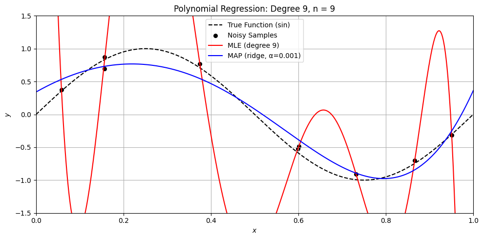
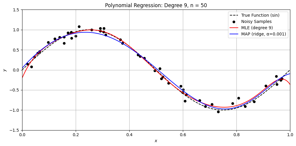
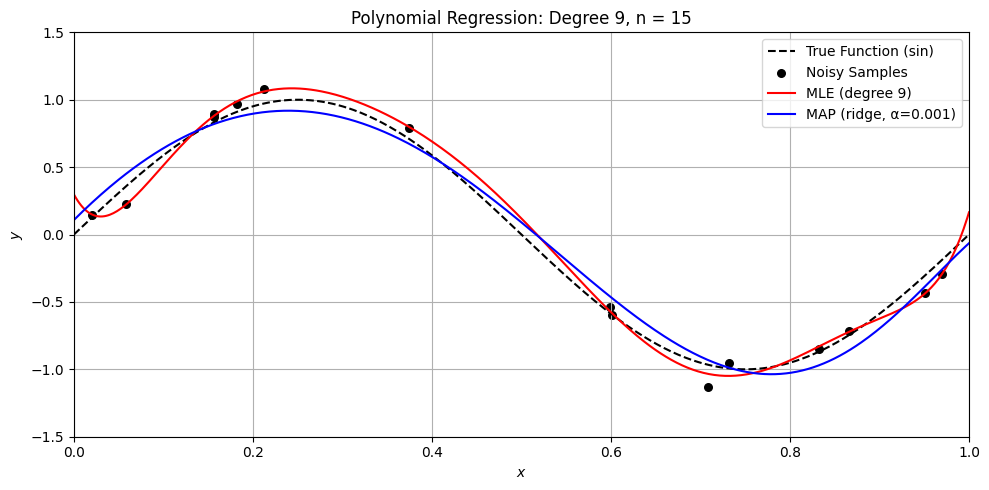
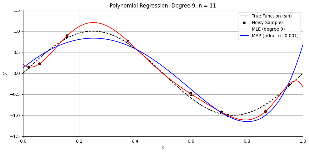
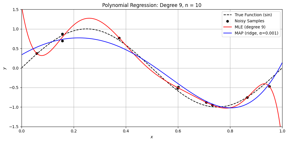
Perfect. Here’s a Python demo that visually compares MLE (ordinary least squares) and MAP (ridge regression) on a small dataset, illustrating:

Overfitting with MLE when \(n \approx d\)
How MAP (ridge) regularizes the solution
Differences in weight magnitude and generalization

Let’s compare MLE and MAP for polynomial regression