Basics of convex functions

Basics of convex functions#

In the remainder of this section, assume $f : \mathbb{R}^d \to \mathbb{R}$ unless otherwise noted. We’ll start with the definitions and then give some results.

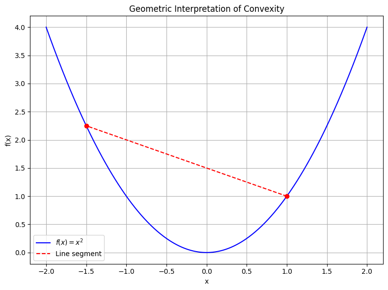
A function $f$ is convex if

\[f(t\mathbf{x} + (1-t)\mathbf{y}) \leq t f(\mathbf{x}) + (1-t)f(\mathbf{y})\]

for all $\mathbf{x}, \mathbf{y} \in \operatorname{dom} f$ and all $t \in [0,1]$.

Geometrically, convexity means that the line segment between two points on the graph of $f$ lies on or above the graph itself.

../_images/0d047f2eca9d0507d4ddae3b984159d8ec13daa6fb1e461bf5913eccdddc8fef.png

If the inequality holds strictly (i.e. $<$ rather than $\leq$) for all $t \in (0,1)$ and $\mathbf{x} \neq \mathbf{y}$, then we say that $f$ is strictly convex.

Strict convexity means that the graph of $f$ lies strictly above the line segment, except at the segment endpoints.

A function $f$ is strongly convex with parameter $m$ (or $m$-strongly convex) if the function

\[\mathbf{x} \mapsto f(\mathbf{x}) - \frac{m}{2}\|\mathbf{x}\|_2^2\]

is convex.

These conditions are given in increasing order of strength; strong convexity implies strict convexity which implies convexity.

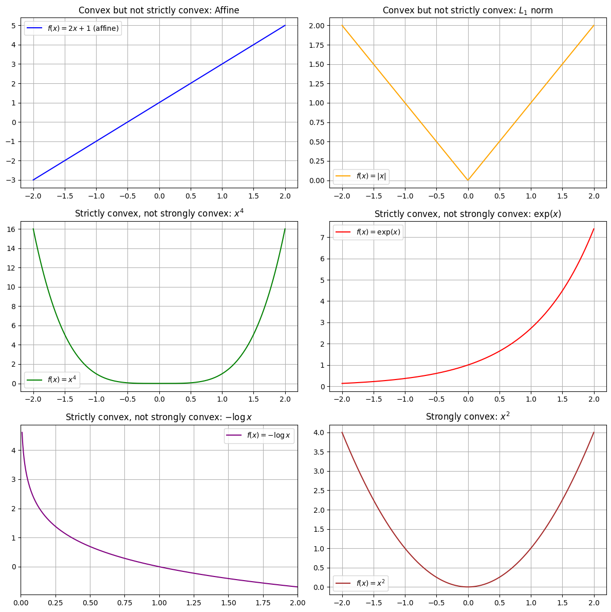
A good way to gain intuition about the distinction between convex, strictly convex, and strongly convex functions is to consider examples where the stronger property fails to hold.

Functions that are convex but not strictly convex:

(i) $f(\mathbf{x}) = \mathbf{w}^{\!\top\!}\mathbf{x} + \alpha$ for any $\mathbf{w} \in \mathbb{R}^d, \alpha \in \mathbb{R}$. Such a function is called an affine function, and it is both convex and concave. (In fact, a function is affine if and only if it is both convex and concave.) Note that linear functions and constant functions are special cases of affine functions.

(ii) $f(\mathbf{x}) = \|\mathbf{x}\|_1$

Functions that are strictly but not strongly convex:

(i) $f(x) = x^4$.

This example is interesting because it is strictly
convex but you cannot show this fact via a second-order argument
(since $f''(0) = 0$).

(ii) $f(x) = \exp(x)$.

This example is interesting because it's bounded
below but has no local minimum.

(iii) $f(x) = -\log x$.

This example is interesting because it's
strictly convex but not bounded below.

Functions that are strongly convex:

(i) $f(\mathbf{x}) = \|\mathbf{x}\|_2^2$

../_images/73b2837986a4347ff42c3215b385f31d9a8f67a8a752328a2e00648d5f330da2.png

Consequences of convexity#

Why do we care if a function is (strictly/strongly) convex?

Basically, our various notions of convexity have implications about the nature of minima. It should not be surprising that the stronger conditions tell us more about the minima.

Proposition (Minima of convex functions)

Let $\mathcal{X}$ be a convex set.

If $f$ is convex, then any local minimum of $f$ in $\mathcal{X}$ is also a global minimum.

Proof. Suppose $f$ is convex, and let $\mathbf{x}^*$ be a local minimum of $f$ in $\mathcal{X}$.

Then for some neighborhood $N \subseteq \mathcal{X}$ about $\mathbf{x}^*$, we have $f(\mathbf{x}) \geq f(\mathbf{x}^*)$ for all $\mathbf{x} \in N$.

Suppose towards a contradiction that there exists $\tilde{\mathbf{x}} \in \mathcal{X}$ such that $f(\tilde{\mathbf{x}}) < f(\mathbf{x}^*)$.

Consider the line segment $\mathbf{x}(t) = t\mathbf{x}^* + (1-t)\tilde{\mathbf{x}}, ~ t \in [0,1]$, noting that $\mathbf{x}(t) \in \mathcal{X}$ by the convexity of $\mathcal{X}$.

Then by the convexity of $f$,

\[f(\mathbf{x}(t)) \leq tf(\mathbf{x}^*) + (1-t)f(\tilde{\mathbf{x}}) < tf(\mathbf{x}^*) + (1-t)f(\mathbf{x}^*) = f(\mathbf{x}^*)\]

for all $t \in (0,1)$.

We can pick $t$ to be sufficiently close to $1$ that $\mathbf{x}(t) \in N$; then $f(\mathbf{x}(t)) \geq f(\mathbf{x}^*)$ by the definition of $N,$ but $f(\mathbf{x}(t)) < f(\mathbf{x}^*)$ by the above inequality, a contradiction.

It follows that $f(\mathbf{x}^*) \leq f(\mathbf{x})$ for all $\mathbf{x} \in \mathcal{X}$, so $\mathbf{x}^*$ is a global minimum of $f$ in $\mathcal{X}$. ◻

Proposition (Minima stricly convex functions)

Let $\mathcal{X}$ be a convex set.

If $f$ is strictly convex, then there exists at most one local minimum of $f$ in $\mathcal{X}$. Consequently, if it exists it is the unique global minimum of $f$ in $\mathcal{X}$.

Proof. The second sentence follows from the first, so all we must show is that if a local minimum exists in $\mathcal{X}$ then it is unique.

Suppose $\mathbf{x}^*$ is a local minimum of $f$ in $\mathcal{X}$, and suppose towards a contradiction that there exists a local minimum $\tilde{\mathbf{x}} \in \mathcal{X}$ such that $\tilde{\mathbf{x}} \neq \mathbf{x}^*$.

Since $f$ is strictly convex, it is convex, so $\mathbf{x}^*$ and $\tilde{\mathbf{x}}$ are both global minima of $f$ in $\mathcal{X}$ by the previous result. Hence $f(\mathbf{x}^*) = f(\tilde{\mathbf{x}})$. Consider the line segment $\mathbf{x}(t) = t\mathbf{x}^* + (1-t)\tilde{\mathbf{x}}, ~ t \in [0,1]$, which again must lie entirely in $\mathcal{X}$. By the strict convexity of $f$,

\[f(\mathbf{x}(t)) < tf(\mathbf{x}^*) + (1-t)f(\tilde{\mathbf{x}}) = tf(\mathbf{x}^*) + (1-t)f(\mathbf{x}^*) = f(\mathbf{x}^*)\]

for all $t \in (0,1)$.

But this contradicts the fact that $\mathbf{x}^*$ is a global minimum. Therefore if $\tilde{\mathbf{x}}$ is a local minimum of $f$ in $\mathcal{X}$, then $\tilde{\mathbf{x}} = \mathbf{x}^*$, so $\mathbf{x}^*$ is the unique minimum in $\mathcal{X}$. ◻

It is worthwhile to examine how the feasible set affects the optimization problem. We will see why the assumption that $\mathcal{X}$ is convex is needed in the results above.

Effects of Changing the Feasible Set#

Consider the function $f(x) = x^2$, which is a strictly convex function. The unique global minimum of this function in $\mathbb{R}$ is $x = 0$.

But let’s see what happens when we change the feasible set $\mathcal{X}$.

../_images/e85eaf769f2592fb17dbfeef407bac2cce3b78cabee44e266e575ab4e7132fe9.png

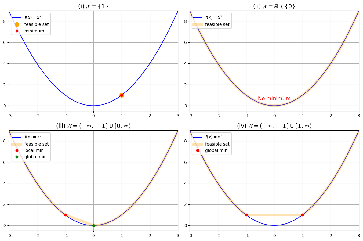
(i) $\mathcal{X} = \{1\}$: This set is actually convex, so we still have a unique global minimum. But it is not the same as the unconstrained minimum!

(ii) $\mathcal{X} = \mathbb{R} \setminus \{0\}$: This set is non-convex, and we can see that $f$ has no minima in $\mathcal{X}$. For any point $x \in \mathcal{X}$, one can find another point $y \in \mathcal{X}$ such that $f(y) < f(x)$.

(iii) $\mathcal{X} = (-\infty,-1] \cup [0,\infty)$: This set is non-convex, and we can see that there is a local minimum ($x = -1$) which is distinct from the global minimum ($x = 0$).

(iv) $\mathcal{X} = (-\infty,-1] \cup [1,\infty)$: This set is non-convex, and we can see that there are two global minima ($x = \pm 1$).

Showing that a function is convex#

Hopefully the previous section has convinced the reader that convexity is an important property. Next we turn to the issue of showing that a function is (strictly/strongly) convex. It is of course possible (in principle) to directly show that the condition in the definition holds, but often this is not the most convenient approach. Instead, we can use a variety of sufficient conditions, properties, and tools—such as the properties of norms, the behavior of the gradient, the use of second derivatives, or by demonstrating that the function is built from convex functions in ways that preserve convexity—to make it much easier to verify convexity in practice.

Proposition (Norms)

Norms are convex.

Proof. Let $\|\cdot\|$ be a norm on a vector space $V$.

Then for all $\mathbf{x}, \mathbf{y} \in V$ and $t \in [0,1]$,

\[\|t\mathbf{x} + (1-t)\mathbf{y}\| \leq \|t\mathbf{x}\| + \|(1-t)\mathbf{y}\| = |t|\|\mathbf{x}\| + |1-t|\|\mathbf{y}\| = t\|\mathbf{x}\| + (1-t)\|\mathbf{y}\|\]

where we have used respectively the triangle inequality, the homogeneity of norms, and the fact that $t$ and $1-t$ are nonnegative.

Hence $\|\cdot\|$ is convex. ◻

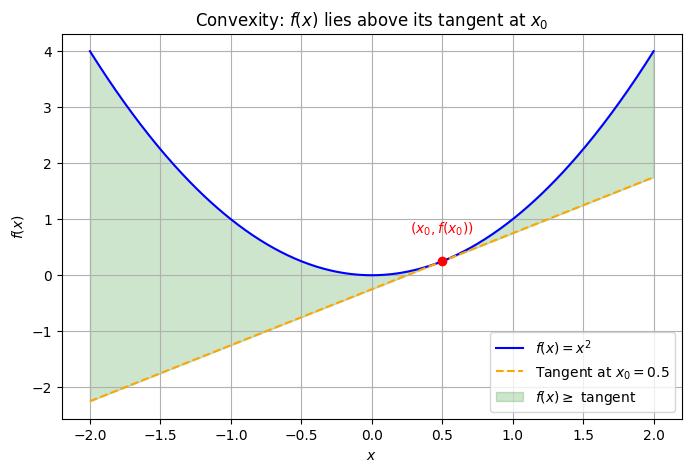
Theorem (First Order Condition for Convex Functions (1D case))

Let $f : \mathbb{R} \to \mathbb{R}$ be differentiable on an open interval $I \subseteq \mathbb{R}$. Then:

$f$ is convex on $I$ if and only if for all $x, y \in I$:

\[ f(y) \geq f(x) + f'(x)(y - x) \]

This means that the graph of $f$ lies above its tangent lines.

🧠 Intuition#

The inequality says: the function at any point $ y $ is at least as large as the linear approximation at $ x $.
This ensures the function is bending upwards — a hallmark of convexity.

../_images/77f1125ccdc379b5ce2bb5fc31926d8463fba37e00908cf1f69498cf602dcef5.png

Proof. (⇒) If $ f $ is convex, then the inequality holds:

Let $ f $ be convex on $ I $.

Fix any $ x, y \in I $, and define the function:

\[ \phi(t) := f((1 - t)x + t y), \quad t \in [0,1]. \]

Since $ f $ is convex, $ \phi $ is convex as a function of $ t $, and differentiable.

By the definition of convexity of a differentiable function on an interval, we have:

\[ \phi(1) \geq \phi(0) + \phi'(0)(1) \]

Compute:

$ \phi(0) = f(x) $
$ \phi(1) = f(y) $
$ \phi'(t) = f'((1 - t)x + t y) \cdot (y - x) \Rightarrow \phi'(0) = f'(x)(y - x) $

Substituting gives:

\[ f(y) \geq f(x) + f'(x)(y - x) \]

(⇐) Conversely, if the inequality holds, then $ f $ is convex:

Let $ x < y $ and $ t \in [0,1] $. Define $ z = (1 - t)x + t y \in [x, y] $. By the hypothesis:

From point $ x $, we have:

\[ f(z) \geq f(x) + f'(x)(z - x) \]

From point $ y $, we also have:

\[ f(z) \geq f(y) + f'(y)(z - y) \]

Now combine this with the mean value theorem and use the inequality on both sides to derive:

\[ f((1 - t)x + t y) \leq (1 - t)f(x) + t f(y) \]

This proves the convexity of $ f $.

Proposition (First Order Condition for Convex Functions)

Suppose $f$ is differentiable.

Then $f$ is convex if and only if

\[f(\mathbf{y}) \geq f(\mathbf{x}) + \langle \nabla f(\mathbf{x}), \mathbf{y} - \mathbf{x} \rangle\]

for all $\mathbf{x}, \mathbf{y} \in \operatorname{dom} f$.

The proposition says that for a convex, differentiable function $f$, the graph of $f$ always lies above its tangent at any point. In other words, the tangent line at any point $x$ is a global underestimator of the function.

Proof. (“Only if” direction)
Suppose $f$ is convex and differentiable.

By the definition of convexity, for any $t \in [0,1]$ and any $\mathbf{x}, \mathbf{y} \in \operatorname{dom} f$,

\[ f(t\mathbf{y} + (1-t)\mathbf{x}) \leq t f(\mathbf{y}) + (1-t) f(\mathbf{x}). \]

Define $\varphi(t) = f(\mathbf{x} + t(\mathbf{y} - \mathbf{x}))$ for $t \in [0,1]$.

Then $\varphi$ is convex as a function of $t$, and differentiable.

The convexity of $\varphi$ implies

\[ \varphi(1) \geq \varphi(0) + \varphi'(0)(1-0) = f(\mathbf{x}) + \langle \nabla f(\mathbf{x}), \mathbf{y} - \mathbf{x} \rangle. \]

But $\varphi(1) = f(\mathbf{y})$, so

\[ f(\mathbf{y}) \geq f(\mathbf{x}) + \langle \nabla f(\mathbf{x}), \mathbf{y} - \mathbf{x} \rangle. \]

(“If” direction)
Suppose the inequality

\[ f(\mathbf{y}) \geq f(\mathbf{x}) + \langle \nabla f(\mathbf{x}), \mathbf{y} - \mathbf{x} \rangle \]

holds for all $\mathbf{x}, \mathbf{y} \in \operatorname{dom} f$.

We want to show that $f$ is convex, i.e.,

\[ f(t\mathbf{y} + (1-t)\mathbf{x}) \leq t f(\mathbf{y}) + (1-t) f(\mathbf{x}) \]

for all $t \in [0,1]$.

Let $t \in (0,1)$ and define $\mathbf{z} = t\mathbf{y} + (1-t)\mathbf{x}$.

By the assumption, applied at $\mathbf{x}$ and $\mathbf{y}$:

\[\begin{split} \begin{aligned} f(\mathbf{y}) &\geq f(\mathbf{z}) + \langle \nabla f(\mathbf{z}), \mathbf{y} - \mathbf{z} \rangle \\ f(\mathbf{x}) &\geq f(\mathbf{z}) + \langle \nabla f(\mathbf{z}), \mathbf{x} - \mathbf{z} \rangle \end{aligned} \end{split}\]

Multiply the first inequality by $t$ and the second by $1-t$, then add:

\[\begin{split} \begin{aligned} t f(\mathbf{y}) + (1-t) f(\mathbf{x}) &\geq t f(\mathbf{z}) + t \langle \nabla f(\mathbf{z}), \mathbf{y} - \mathbf{z} \rangle \\ &\quad + (1-t) f(\mathbf{z}) + (1-t) \langle \nabla f(\mathbf{z}), \mathbf{x} - \mathbf{z} \rangle \\ &= f(\mathbf{z}) + \langle \nabla f(\mathbf{z}), t(\mathbf{y} - \mathbf{z}) + (1-t)(\mathbf{x} - \mathbf{z}) \rangle \end{aligned} \end{split}\]

But

\[\begin{split} \begin{aligned} t(\mathbf{y} - \mathbf{z}) + (1-t)(\mathbf{x} - \mathbf{z}) &= t(\mathbf{y} - (t\mathbf{y} + (1-t)\mathbf{x})) + (1-t)(\mathbf{x} - (t\mathbf{y} + (1-t)\mathbf{x})) \\ &= t((1-t)(\mathbf{y} - \mathbf{x})) + (1-t)(-t(\mathbf{y} - \mathbf{x})) \\ &= t(1-t)(\mathbf{y} - \mathbf{x}) - t(1-t)(\mathbf{y} - \mathbf{x}) \\ &= 0 \end{aligned} \end{split}\]

So the inner product term vanishes, and we have

\[ t f(\mathbf{y}) + (1-t) f(\mathbf{x}) \geq f(\mathbf{z}) = f(t\mathbf{y} + (1-t)\mathbf{x}) \]

which is the definition of convexity.

◻

Proposition (Hessian of Convex Functions)

Suppose $f$ is twice differentiable.

Then

(i) $f$ is convex if and only if $\nabla^2 f(\mathbf{x}) \succeq 0$ for all $\mathbf{x} \in \operatorname{dom} f$.

(ii) If $\nabla^2 f(\mathbf{x}) \succ 0$ for all $\mathbf{x} \in \operatorname{dom} f$, then $f$ is strictly convex.

(iii) $f$ is $m$-strongly convex if and only if $\nabla^2 f(\mathbf{x}) \succeq mI$ for all $\mathbf{x} \in \operatorname{dom} f$.

This proposition provides a simple way to check convexity, strict convexity, and strong convexity for twice differentiable functions by looking at the Hessian matrix $\nabla^2 f(\mathbf{x})$:

If the Hessian is positive semidefinite everywhere (all eigenvalues are nonnegative), the function is convex.
If the Hessian is positive definite everywhere (all eigenvalues are strictly positive), the function is strictly convex.
If the Hessian is bounded below by $mI$ (all eigenvalues are at least $m > 0$), the function is $m$-strongly convex.

These conditions are very useful in practice, because checking the Hessian is often easier than checking the definition of convexity directly.

Proof. We prove each part in turn.

(i) $f$ is convex if and only if $\nabla^2 f(\mathbf{x}) \succeq 0$ for all $\mathbf{x}$.

Recall that for a twice differentiable function $f$, the second-order Taylor expansion at $\mathbf{x}$ gives

\[ f(\mathbf{y}) = f(\mathbf{x}) + \langle \nabla f(\mathbf{x}), \mathbf{y} - \mathbf{x} \rangle + \frac{1}{2} (\mathbf{y} - \mathbf{x})^\top \nabla^2 f(\mathbf{z}) (\mathbf{y} - \mathbf{x}) \]

for some $\mathbf{z}$ on the line segment between $\mathbf{x}$ and $\mathbf{y}$.

($\implies$) Suppose $f$ is convex.

Then, by the first-order condition for convexity, for all $\mathbf{x}, \mathbf{y}$,

\[ f(\mathbf{y}) \geq f(\mathbf{x}) + \langle \nabla f(\mathbf{x}), \mathbf{y} - \mathbf{x} \rangle. \]

Subtracting the right-hand side from the Taylor expansion, we get

\[ f(\mathbf{y}) - f(\mathbf{x}) - \langle \nabla f(\mathbf{x}), \mathbf{y} - \mathbf{x} \rangle = \frac{1}{2} (\mathbf{y} - \mathbf{x})^\top \nabla^2 f(\mathbf{z}) (\mathbf{y} - \mathbf{x}) \geq 0 \]

for all $\mathbf{x}, \mathbf{y}$ and some $\mathbf{z}$ between them. This is only possible if $\nabla^2 f(\mathbf{z})$ is positive semidefinite for all $\mathbf{z}$, and thus for all $\mathbf{x}$.

($\impliedby$) Conversely, suppose $\nabla^2 f(\mathbf{x}) \succeq 0$ for all $\mathbf{x}$.

We want to prove that this implies $f$ is convex.

Let $\mathbf{x}, \mathbf{y} \in \operatorname{dom} f$, and define the function $\phi(t) = f(\mathbf{x} + t(\mathbf{y} - \mathbf{x}))$ for $t \in [0,1]$.

This is the restriction of $f$ to the line segment between $\mathbf{x}$ and $\mathbf{y}$, i.e., a function from $\mathbb{R} \to \mathbb{R}$.

Then $\phi$ is twice differentiable with:

\[ \phi'(t) = \nabla f(\mathbf{x}_t)^\top (\mathbf{y} - \mathbf{x}), \quad \text{and} \quad \phi''(t) = (\mathbf{y} - \mathbf{x})^\top \nabla^2 f(\mathbf{x}_t) (\mathbf{y} - \mathbf{x}), \]

where $\mathbf{x}_t = \mathbf{x} + t(\mathbf{y} - \mathbf{x})$. By assumption, $\nabla^2 f(\mathbf{x}_t) \succeq 0$, so:

\[ \phi''(t) \geq 0 \quad \text{for all } t \in [0,1]. \]

Hence, $\phi$ is a convex function on $[0,1]$, and so:

\[ f(t\mathbf{y} + (1 - t)\mathbf{x}) = \phi(t) \leq (1 - t)\phi(0) + t\phi(1) = (1 - t)f(\mathbf{x}) + t f(\mathbf{y}), \]

which shows that $f$ is convex.

(ii) If $\nabla^2 f(\mathbf{x}) \succ 0$ for all $\mathbf{x}$, then $f$ is strictly convex.

If $\nabla^2 f(\mathbf{x})$ is positive definite for all $\mathbf{x}$, then for any $\mathbf{x} \neq \mathbf{y}$, the quadratic form $(\mathbf{y} - \mathbf{x})^\top \nabla^2 f(\mathbf{z}) (\mathbf{y} - \mathbf{x}) > 0$ for all $\mathbf{z}$ between $\mathbf{x}$ and $\mathbf{y}$.

Thus, the Taylor expansion above is strictly greater than zero for $\mathbf{x} \neq \mathbf{y}$, so the convexity inequality is strict for $t \in (0,1)$, i.e., $f$ is strictly convex.

(iii) $f$ is $m$-strongly convex if and only if $\nabla^2 f(\mathbf{x}) \succeq mI$ for all $\mathbf{x}$.

Recall that $f$ is $m$-strongly convex if $f(\mathbf{x}) - \frac{m}{2}\|\mathbf{x}\|^2$ is convex.

The Hessian of this function is $\nabla^2 f(\mathbf{x}) - mI$. By part (i), this is convex if and only if $\nabla^2 f(\mathbf{x}) - mI \succeq 0$, i.e., $\nabla^2 f(\mathbf{x}) \succeq mI$ for all $\mathbf{x}$.

◻

The following propositions show how convexity is preserved under scaling and addition of functions.

Proposition (Scaling Convex Functions)

If $f$ is convex and $\alpha \geq 0$, then $\alpha f$ is convex.

Proof. Suppose $f$ is convex and $\alpha \geq 0$.

Then for all $\mathbf{x}, \mathbf{y} \in \operatorname{dom}(\alpha f) = \operatorname{dom} f$,

\[\begin{split}\begin{aligned} (\alpha f)(t\mathbf{x} + (1-t)\mathbf{y}) &= \alpha f(t\mathbf{x} + (1-t)\mathbf{y}) \\ &\leq \alpha\left(tf(\mathbf{x}) + (1-t)f(\mathbf{y})\right) \\ &= t(\alpha f(\mathbf{x})) + (1-t)(\alpha f(\mathbf{y})) \\ &= t(\alpha f)(\mathbf{x}) + (1-t)(\alpha f)(\mathbf{y}) \end{aligned}\end{split}\]

so $\alpha f$ is convex. ◻

Proposition (Sum of Convex Functions)

If $f$ and $g$ are convex, then $f+g$ is convex.

Furthermore, if $g$ is strictly convex, then $f+g$ is strictly convex.

If $g$ is $m$-strongly convex, then $f+g$ is $m$-strongly convex.

Proof. Suppose $f$ and $g$ are convex.

Then for all $\mathbf{x}, \mathbf{y} \in \operatorname{dom} (f+g) = \operatorname{dom} f \cap \operatorname{dom} g$,

\[\begin{split}\begin{aligned} (f+g)(t\mathbf{x} + (1-t)\mathbf{y}) &= f(t\mathbf{x} + (1-t)\mathbf{y}) + g(t\mathbf{x} + (1-t)\mathbf{y}) \\ &\leq tf(\mathbf{x}) + (1-t)f(\mathbf{y}) + g(t\mathbf{x} + (1-t)\mathbf{y}) & \text{convexity of $f$} \\ &\leq tf(\mathbf{x}) + (1-t)f(\mathbf{y}) + tg(\mathbf{x}) + (1-t)g(\mathbf{y}) & \text{convexity of $g$} \\ &= t(f(\mathbf{x}) + g(\mathbf{x})) + (1-t)(f(\mathbf{y}) + g(\mathbf{y})) \\ &= t(f+g)(\mathbf{x}) + (1-t)(f+g)(\mathbf{y}) \end{aligned}\end{split}\]

so $f + g$ is convex.

If $g$ is strictly convex, the second inequality above holds strictly for $\mathbf{x} \neq \mathbf{y}$ and $t \in (0,1)$, so $f+g$ is strictly convex.

If $g$ is $m$-strongly convex, then the function $h(\mathbf{x}) \equiv g(\mathbf{x}) - \frac{m}{2}\|\mathbf{x}\|_2^2$ is convex, so $f+h$ is convex.

But

\[(f+h)(\mathbf{x}) \equiv f(\mathbf{x}) + h(\mathbf{x}) \equiv f(\mathbf{x}) + g(\mathbf{x}) - \frac{m}{2}\|\mathbf{x}\|_2^2 \equiv (f+g)(\mathbf{x}) - \frac{m}{2}\|\mathbf{x}\|_2^2\]

so $f+g$ is $m$-strongly convex. ◻

Proposition (Weighted Sum of Convex Functions)

If $f_1, \dots, f_n$ are convex and $\alpha_1, \dots, \alpha_n \geq 0$, then

\[\sum_{i=1}^n \alpha_i f_i\]

is convex.

Proof. Follows from the previous two propositions by induction. ◻

A common way to generate new convex functions is by composing a convex function with an affine transformation, as stated in the following proposition:

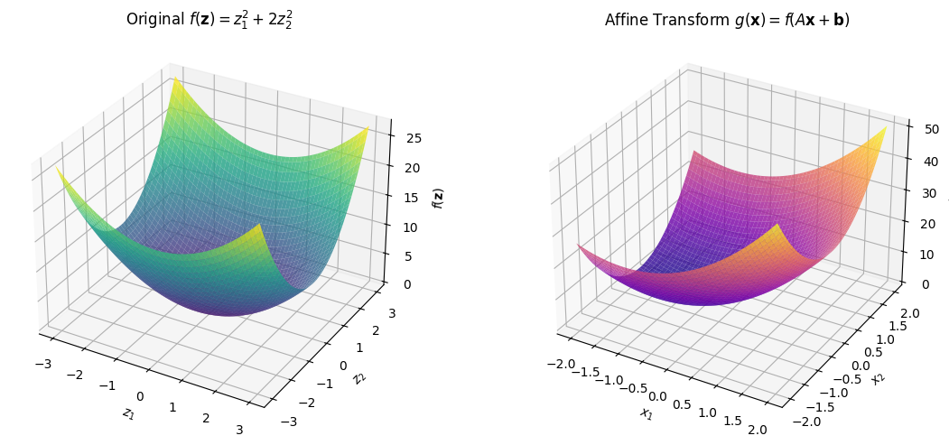
Proposition (Combination of Affine and Convex Functions)

If $f$ is convex, then $g(\mathbf{x}) \equiv f(\mathbf{A}\mathbf{x} + \mathbf{b})$ is convex for any appropriately-sized $\mathbf{A}$ and $\mathbf{b}$.

The following plot demonstrates how composing a convex function with an affine transformation preserves convexity: the left plot shows the original convex function, and the right plot shows its affine transformation.

../_images/7f5ee29966a1ce90a5a74196d7eca24d5ab06b165f6800a71640363f78cdb068.png

Proof. Suppose $f$ is convex and $g$ is defined like so.

Then for all $\mathbf{x}, \mathbf{y} \in \operatorname{dom} g$,

\[\begin{split}\begin{aligned} g(t\mathbf{x} + (1-t)\mathbf{y}) &= f(\mathbf{A}(t\mathbf{x} + (1-t)\mathbf{y}) + \mathbf{b}) \\ &= f(t\mathbf{A}\mathbf{x} + (1-t)\mathbf{A}\mathbf{y} + \mathbf{b}) \\ &= f(t\mathbf{A}\mathbf{x} + (1-t)\mathbf{A}\mathbf{y} + t\mathbf{b} + (1-t)\mathbf{b}) \\ &= f(t(\mathbf{A}\mathbf{x} + \mathbf{b}) + (1-t)(\mathbf{A}\mathbf{y} + \mathbf{b})) \\ &\leq tf(\mathbf{A}\mathbf{x} + \mathbf{b}) + (1-t)f(\mathbf{A}\mathbf{y} + \mathbf{b}) & \text{convexity of $f$} \\ &= tg(\mathbf{x}) + (1-t)g(\mathbf{y}) \end{aligned}\end{split}\]

Thus $g$ is convex. ◻

Proposition (Maximum of Convex Functions)

If $f$ and $g$ are convex, then $h(\mathbf{x}) \equiv \max\{f(\mathbf{x}), g(\mathbf{x})\}$ is convex.

Let’s look at two convex functions and their pointwise maximum. The resulting function will be convex, but may not be smooth where the two functions cross.

../_images/74c35c292df4be8b1d822ca65e515482999b1926d6f61071fb3b11672a33c1d8.png

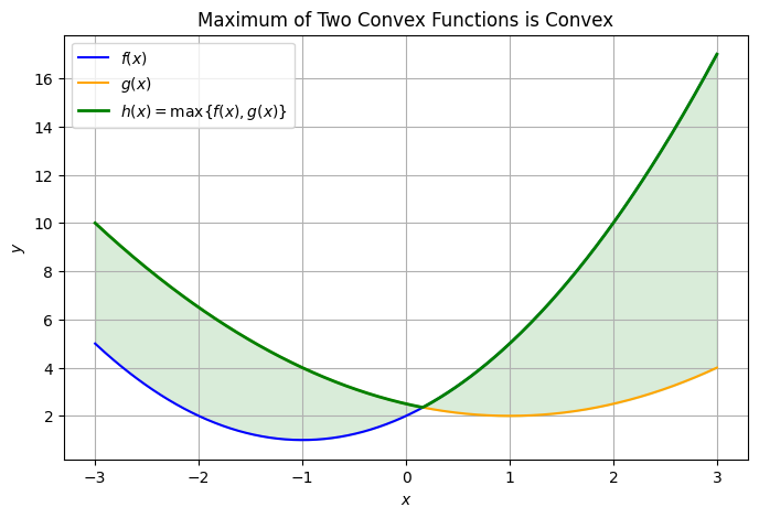
The blue and orange curves are two convex functions.
The green curve is their pointwise maximum, which is also convex (but not necessarily smooth everywhere).
The shaded region highlights the “upper envelope” formed by the maximum.

Proof. Suppose $f$ and $g$ are convex and $h$ is defined like so. Then for all $\mathbf{x}, \mathbf{y} \in \operatorname{dom} h$,

\[\begin{split}\begin{aligned} h(t\mathbf{x} + (1-t)\mathbf{y}) &= \max\{f(t\mathbf{x} + (1-t)\mathbf{y}), g(t\mathbf{x} + (1-t)\mathbf{y})\} \\ &\leq \max\{tf(\mathbf{x}) + (1-t)f(\mathbf{y}), tg(\mathbf{x}) + (1-t)g(\mathbf{y})\} \\ &\leq \max\{tf(\mathbf{x}), tg(\mathbf{x})\} + \max\{(1-t)f(\mathbf{y}), (1-t)g(\mathbf{y})\} \\ &= t\max\{f(\mathbf{x}), g(\mathbf{x})\} + (1-t)\max\{f(\mathbf{y}), g(\mathbf{y})\} \\ &= th(\mathbf{x}) + (1-t)h(\mathbf{y}) \end{aligned}\end{split}\]

Note that in the first inequality we have used convexity of $f$ and $g$ plus the fact that

\[a \leq c, \; b \leq d \quad \implies \quad \max\{a,b\} \leq \max\{c,d\}.\]

In the second inequality we have used the fact that $\max\{a+b, c+d\} \leq \max\{a,c\} + \max\{b,d\}$.

Thus $h$ is convex. ◻

Convexity and Gradient Descent Convergence#

Gradient descent is one of the most widely used optimization methods in machine learning. Its behavior is closely tied to the convexity of the objective function.

Gradient Descent Algorithm#

Given a differentiable function $f: \mathbb{R}^d \to \mathbb{R}$, the gradient descent update rule is:

\[ \mathbf{x}^{(k+1)} = \mathbf{x}^{(k)} - \eta \nabla f(\mathbf{x}^{(k)}) \]

where:

$\eta > 0$ is the learning rate (step size),
$\nabla f(\mathbf{x})$ is the gradient at $\mathbf{x}$.

Why Convexity Matters#

1. Convex functions:#

If $f$ is convex and differentiable, then any local minimum is a global minimum. Gradient descent will eventually reach a minimizer — but convergence may be slow and can depend on the conditioning of the problem.

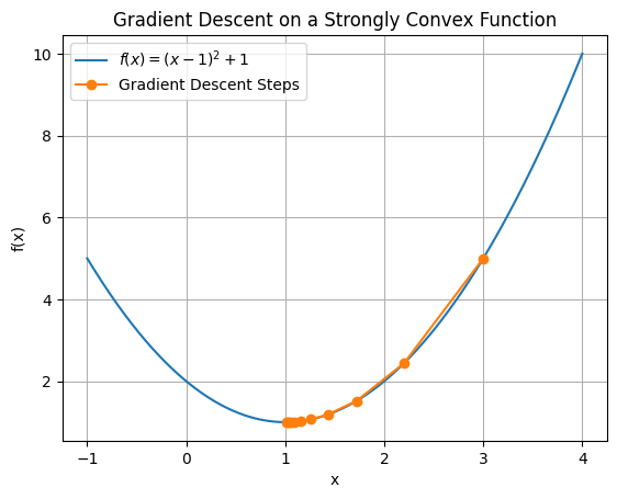
2. Strongly convex functions:#

If $f$ is $\mu$-strongly convex and has L-Lipschitz continuous gradients, then gradient descent converges linearly to the global minimizer $\mathbf{x}^*$, meaning:

\[ f(\mathbf{x}^{(k)}) - f(\mathbf{x}^*) \leq \left(1 - \eta \mu\right)^k \left(f(\mathbf{x}^{(0)}) - f(\mathbf{x}^*)\right) \]

for $\eta \in \left(0, \frac{2}{L} \right)$.

→ The stronger the curvature, the faster the convergence.

../_images/04e41a3771982c891de4f46aeede783d31e9932a52aa23ee72304f78fa83c5fa.png

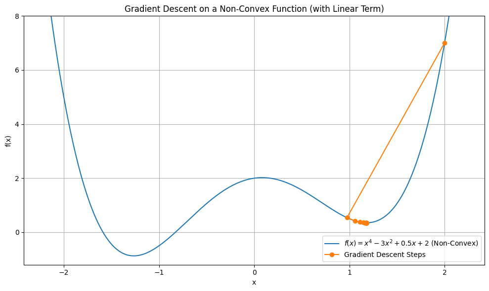
However, non-convex functions may have multiple local minima. Thus, gradient descent may get stuck in a local minimum.

../_images/e03392b4dcbb7d43863f7f0465170a2d7a0d231004dfa15557874fdd45aabe89.png

\[ f(x) = x^4 - 3x^2 + 0.5x + 2 \]

Machine Learning Objectives and Convexity#

✅ 1. Linear Regression with Squared Loss#

Problem: Fit a linear model $y = X\beta + \varepsilon$ using ordinary least squares (OLS).

Loss function:

\[ L(\beta) = \frac{1}{2} \|X\beta - y\|^2 \]

This loss function is strongly convex when $X^\top X$ is full rank.
Guarantees a unique global minimum.

✅ 2. Ridge Regression#

Loss function:

\[ L(\beta) = \frac{1}{2} \|X\beta - y\|^2 + \lambda \|\beta\|^2 \]

The regularization term $\lambda \|\beta\|^2$ makes the loss strongly convex even if $X^\top X$ is not full rank.

✅ 3. Logistic Regression (Binary Classification)#

Loss function:

\[ L(\beta) = \sum_{i=1}^n \log\left(1 + \exp(-y_i X_i^\top \beta)\right) \]

Convex but not strongly convex unless regularized.

❌ 4. Two-Layer Neural Network#

Loss function:

\[ L(W_1, W_2, b_1, b_2) = \frac{1}{2n} \sum_{i=1}^n \left( W_2 \cdot \tanh(W_1 x_i + b_1) + b_2 - y_i \right)^2 \]

Not convex in the weights due to nonlinear activation.
Shows multiple minima and complex curvature.
Requires careful initialization, learning rate tuning, and often benefits from regularization.

Here is a visualization of the non-convex loss surface of a simple 2-layer neural network with architecture:

\[ \hat{y} = W_2 \cdot \tanh(W_1 x + b_1) + b_2 \]

Show code cell source Hide code cell source

import numpy as np
import matplotlib.pyplot as plt
from mpl_toolkits.mplot3d import Axes3D

# Simulate simple 1D regression data
np.random.seed(0)
n = 50
x = np.linspace(-2, 2, n).reshape(-1, 1)
y = 2 * np.sin(1.5 * x) + 0.3 * np.random.randn(n, 1)

# Define a 2-layer neural network model manually
def two_layer_nn(x, w):
    W1 = w[0]
    b1 = w[1]
    W2 = w[2]
    b2 = w[3]
    h = np.tanh(W1 * x + b1)
    return W2 * h + b2

# Loss function for a grid of parameters (varying W1 and W2, fixing biases)
w1_range = np.linspace(-2, 3, 100)
w2_range = np.linspace(-2, 3, 100)
loss_grid = np.zeros((len(w1_range), len(w2_range)))

for i, w1 in enumerate(w1_range):
    for j, w2 in enumerate(w2_range):
        preds = two_layer_nn(x, [w1, 0.0, w2, 0.0])
        loss_grid[j, i] = np.mean((preds - y)**2)

# Plot the non-convex loss landscape
W1, W2 = np.meshgrid(w1_range, w2_range)

# Initialize gradient descent at a random point
w1_gd, w2_gd = [-1], [2.9]
eta = 0.05  # learning rate

# Approximate gradient via finite differences
def compute_loss(w1, w2):
    preds = two_layer_nn(x, [w1, 0.0, w2, 0.0])
    return np.mean((preds - y)**2)

for _ in range(30):
    w1, w2 = w1_gd[-1], w2_gd[-1]
    eps = 1e-4
    grad_w1 = (compute_loss(w1 + eps, w2) - compute_loss(w1 - eps, w2)) / (2 * eps)
    grad_w2 = (compute_loss(w1, w2 + eps) - compute_loss(w1, w2 - eps)) / (2 * eps)
    w1_gd.append(w1 - eta * grad_w1)
    w2_gd.append(w2 - eta * grad_w2)

# Compute loss values along the path
loss_gd = [compute_loss(w1, w2) for w1, w2 in zip(w1_gd, w2_gd)]

# Overlay gradient descent path on 3D surface
fig = plt.figure(figsize=(10, 7))
ax = fig.add_subplot(111, projection='3d')
ax.plot_surface(W1, W2, loss_grid, cmap="viridis", edgecolor='none', alpha=0.6)
ax.plot(w1_gd, w2_gd, loss_gd, 'ro-', label='Gradient Descent Path')
ax.set_title("Gradient Descent Path on 3D Loss Surface")
ax.set_xlabel("Weight W1")
ax.set_ylabel("Weight W2")
ax.set_zlabel("Loss")
# ax.set_zlim([0,12])
# ax.set_xlim([-2,4.6])
ax.legend()
plt.tight_layout()
plt.show()

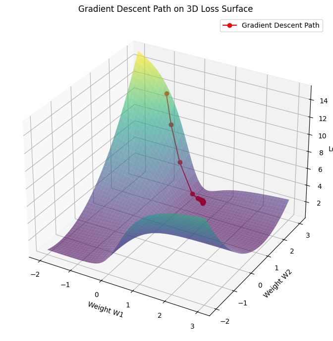
../_images/5afaf86ad741d2b5c1a468b19f5cff72f0463ebd08f3a5219b64d1c76a4e93f2.png

We fixed biases $b_1 = b_2 = 0$ and varied the weights $W_1$ and $W_2$.

The loss landscape shows:

Multiple local minima and saddle points.
Wiggly, non-convex behavior characteristic of neural networks, even with a single hidden unit.

This 3D plot shows the gradient descent trajectory over the non-convex loss surface of the 2-layer neural network:

The red path illustrates how optimization progresses from the initial point $(W_1, W_2) = (-1.0, 2.9)$.
The descent gets pulled into a local valley, which may not be the global minimum.
This visual underscores the complexity of optimizing neural networks, especially compared to convex problems.

Basics of convex functions

Contents

Basics of convex functions#

Consequences of convexity#

Effects of Changing the Feasible Set#

Showing that a function is convex#

🧠 Intuition#

(⇐) Conversely, if the inequality holds, then \( f \) is convex:

Convexity and Gradient Descent Convergence#

Gradient Descent Algorithm#

Why Convexity Matters#

1. Convex functions:#

2. Strongly convex functions:#

Machine Learning Objectives and Convexity#

✅ 1. Linear Regression with Squared Loss#

✅ 2. Ridge Regression#

✅ 3. Logistic Regression (Binary Classification)#

❌ 4. Two-Layer Neural Network#