Eigenvalues and Eigenvectors

Eigenvalues and Eigenvectors#

For a square matrix \(\mathbf{A} \in \mathbb{R}^{n \times n}\), there may be vectors which, when \(\mathbf{A}\) is applied to them, are simply scaled by some constant.

A nonzero vector \(\mathbf{x} \in \mathbb{C}^n\) is an eigenvector of \(\mathbf{A}\) corresponding to eigenvalue \(\lambda \in \mathbb{C}\) if

\[\mathbf{A}\mathbf{x} = \lambda\mathbf{x}\]

The zero vector is excluded from this definition because \(\mathbf{A}\mathbf{0} = \mathbf{0} = \lambda\mathbf{0}\) for every \(\lambda\).

Eigenvalues and eigenvectors can be complex numbers, even if \(\mathbf{A}\) is real-valued. We will provide a high-level discussion of the conditions below.

First, let’s look at an example and how multiplication with a matrix \(\mathbf{A}\) transforms vectors that lie on the unit circle and, in particular, how it changes it’s eivenvectors during multiplication.

\[\begin{split} \mathbf{A} = \begin{pmatrix}1.5 & 0.5 \\ 0.1 & 1.2\end{pmatrix} \end{split}\]

The matrix has Eigenvalues λ₁ = 1.62, λ₂ = 1.08.

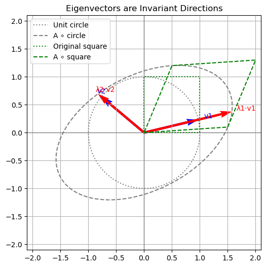
../_images/d6d04f98b0b7036e0c334dad45f7ec7d32e59332dda5f83f0cb24274fad41247.png

The visualization shows:

The original unit circle (dashed black)
The transformed unit circle under \(\mathbf{A}\) (solid red)
The eigenvectors in blue and their scaled images in green

Note how the eigenvectors are aligned with the directions that remain unchanged in orientation under transformation — they are only scaled by their respective eigenvalues.

Eigenvectors can be real-valued or complex.#

Here’s a breakdown of the geometric distinction between linear maps that have only real eigenvectors and those that have complex eigenvectors:

Real Eigenvectors → Maps That Stretch or Reflect Along Fixed Directions#

If a matrix \(\mathbf{A} \in \mathbb{R}^{n \times n}\) has only real eigenvalues and eigenvectors, it means:

There exist real directions in space that are preserved (up to scaling).
The action of the matrix is intuitively:
- Scaling (positive eigenvalues)
- Reflection + scaling (negative eigenvalues)
You can visualize this as:
- Pulling/stretching space along certain axes
- Possibly flipping directions

Complex Eigenvectors → Maps That Rotate or Spiral#

If a matrix has complex eigenvalues and no real eigenvectors, it cannot leave any real direction invariant.

This typically corresponds to:

Rotation or spiral motion
Sometimes rotation + scaling (when complex eigenvalues have modulus \(\ne 1\))
The action in real space:
- No real eigenvector
- Points are rotated or rotated and scaled
- Repeated application creates circular or spiraling trajectories

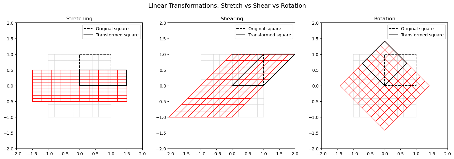
Example: Stretching vs. Shearing vs. Rotation#

Stretching: scales space differently along the axes. The matrix has only real eigenvalues and eigenvectors.
Shearing: shifts one axis direction while keeping the other fixed. The matrix has only real eigenvalues and eigenvectors.
Rotation: turns everything around the origin. The matrix has only complex eigenvalues and eigenvectors.

Each transformation is applied to a unit square and a grid, so you can clearly see how space is deformed under each linear map.

../_images/7cb620d5899a876b48a7912b7167199ee6e3fc48ddba83f74f522daeb4c1922e.png

We now give some useful results about how eigenvalues change after various manipulations.

Proposition (Eigenvalues and Eigenvectors)

Let \(\mathbf{x}\) be an eigenvector of \(\mathbf{A}\) with corresponding eigenvalue \(\lambda\).

Then

(i) For any \(\gamma \in \mathbb{R}\), \(\mathbf{x}\) is an eigenvector of \(\mathbf{A} + \gamma\mathbf{I}\) with eigenvalue \(\lambda + \gamma\).

(ii) If \(\mathbf{A}\) is invertible, then \(\mathbf{x}\) is an eigenvector of \(\mathbf{A}^{-1}\) with eigenvalue \(\lambda^{-1}\).

(iii) \(\mathbf{A}^k\mathbf{x} = \lambda^k\mathbf{x}\) for any \(k \in \mathbb{Z}\) (where \(\mathbf{A}^0 = \mathbf{I}\) by definition).

Below we illustrate the geometric meaning of Propositions (i)–(iii) using the same original matrix \(\mathbf{A}\).

Each subplot shows:

The unit circle (dashed black)
The circle transformed by the original matrix \(\mathbf{A}\) (dotted gray)
The circle transformed by the modified matrix (solid red)
An eigenvector of \(\mathbf{A}\) (blue)
The eigenvector after transformation by the modified matrix (red arrow)

Show code cell source Hide code cell source

import numpy as np
import matplotlib.pyplot as plt

def plot_eig_effect(ax, A_original, A_transformed, transformation_label, proposition_label, color_vec='red', color_circle='crimson',):
    # Unit circle
    theta = np.linspace(0, 2 * np.pi, 200)
    circle = np.vstack((np.cos(theta), np.sin(theta)))
    circle_A = A_original @ circle
    circle_transformed = A_transformed @ circle

    # Eigenvectors and values of A_original
    eigvals, eigvecs = np.linalg.eig(A_original)

    # Plot unit and transformed circles
    ax.plot(circle[0], circle[1], 'k--', label='Unit Circle')
    ax.plot(circle_A[0], circle_A[1], color='gray', linestyle=':', label='A ∘ Circle')
    ax.plot(circle_transformed[0], circle_transformed[1], color=color_circle, label=transformation_label+' ∘ Circle')

    for i in range(2):
        v = eigvecs[:, i]
        v = v / np.linalg.norm(v)
        Atrans_v = A_transformed @ v

        # Plot eigenvector and its transformed image
        ax.quiver(0, 0, v[0], v[1], angles='xy', scale_units='xy', scale=1, color='blue', label=r'Eigenvector $\mathbf{v}$' if i == 0 else None)
        ax.quiver(0, 0, Atrans_v[0], Atrans_v[1], angles='xy', scale_units='xy', scale=1, color=color_vec, label=transformation_label+r' ∘ $\mathbf{v}$' if i == 0 else None)

    # Formatting
    ax.set_xlim(-3, 3)
    ax.set_ylim(-3, 3)
    ax.set_aspect('equal')
    ax.axhline(0, color='gray', lw=0.5)
    ax.axvline(0, color='gray', lw=0.5)
    ax.set_title(proposition_label + transformation_label)
    ax.grid(True)

# --- Base matrix ---
A = np.array([[1.5, 0.5],
              [0.1, 1.2]])

# --- Matrix variants ---
gamma = 0.5
A_shifted = A + gamma * np.eye(2)
A_inv = np.linalg.inv(A)
A_sq = A @ A

# --- Plotting ---
fig, axes = plt.subplots(1, 3, figsize=(18, 6))

plot_eig_effect(axes[0], A, A_shifted, "(A + γI)", proposition_label= "i): ")
plot_eig_effect(axes[1], A, A_inv, "A⁻¹", proposition_label= "ii): ")
plot_eig_effect(axes[2], A, A_sq, "A²", proposition_label= "iii): ")

for ax in axes:
    ax.legend()

plt.suptitle("Eigenvector Transformations for Proposition (i)–(iii)", fontsize=16)
plt.tight_layout(rect=[0, 0, 1, 0.95])
plt.show()

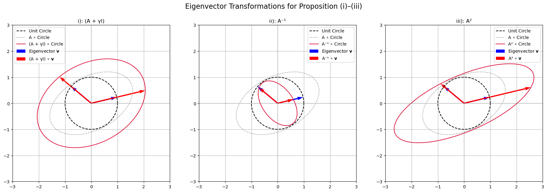
../_images/fd4c4818690df6f295ddba6702e6261fb22c1b8dcbed13e2762e14432dec086c.png

We observe that:

The eigenvector direction is invariant (it doesn’t rotate)
The scaling changes depending on the transformation:
- In (i), \(\mathbf{A} + \gamma \mathbf{I}\) adds \(\gamma\) to the eigenvalue.
- In (ii), \(\mathbf{A}^{-1}\) inverts the eigenvalue.
- In (iii), \(\mathbf{A}^2\) squares the eigenvalue.

Note how the red-transformed circles deform differently in each panel, but the eigenvector stays aligned.

Proof. (i) follows readily:

\[(\mathbf{A} + \gamma\mathbf{I})\mathbf{x} = \mathbf{A}\mathbf{x} + \gamma\mathbf{I}\mathbf{x} = \lambda\mathbf{x} + \gamma\mathbf{x} = (\lambda + \gamma)\mathbf{x}\]

(ii) Suppose \(\mathbf{A}\) is invertible. Then

\[\mathbf{x} = \mathbf{A}^{-1}\mathbf{A}\mathbf{x} = \mathbf{A}^{-1}(\lambda\mathbf{x}) = \lambda\mathbf{A}^{-1}\mathbf{x}\]

Dividing by \(\lambda\), which is valid because the invertibility of \(\mathbf{A}\) implies \(\lambda \neq 0\), gives \(\lambda^{-1}\mathbf{x} = \mathbf{A}^{-1}\mathbf{x}\).

(iii) The case \(k \geq 0\) follows immediately by induction on \(k\). Then the general case \(k \in \mathbb{Z}\) follows by combining the \(k \geq 0\) case with (ii). ◻

Relationship between Eigenvalues and Determinant#

Interestingly, the determinant of a matrix is equal to the product of its eigenvalues (repeated according to multiplicity):

\[\det(\mathbf{A}) = \prod_{i=1}^n \lambda_i(\mathbf{A})\]

This provides a means to find the eigenvalues by deriving the roots of the characteristic polynomial.

Corollary (Characteristic Polynomial)

The eigenvalues of a matrix \(\mathbf{A} \in \mathbb{R}^{n \times n}\) are the roots of its characteristic polynomial defined as:

\[ p(\lambda) = \det(\mathbf{A} - \lambda \mathbf{I}) \]

It is a degree-\(n\) polynomial in \(\lambda\), and its roots are precisely the eigenvalues of \(\mathbf{A}\).

Proof. Characteristic Polynomial

By definition, \(\lambda\) is an eigenvalue of \(\mathbf{A}\) if:

\[ \exists \, \mathbf{x} \neq \mathbf{0} \text{ such that } \mathbf{A} \mathbf{x} = \lambda \mathbf{x} \]

Rewriting:

\[ (\mathbf{A} - \lambda \mathbf{I}) \mathbf{x} = \mathbf{0} \]

This is a homogeneous linear system. A nontrivial solution exists if and only if the matrix \(\mathbf{A} - \lambda \mathbf{I}\) is not invertible, which according to the fundamental equivalences for square matrices is equivalent to:

\[ \det(\mathbf{A} - \lambda \mathbf{I}) = 0 \]

Therefore, the eigenvalues are the roots of the characteristic polynomial \(p(\lambda)\).

\[\begin{split} \mathbf{A} - \lambda \mathbf{I} = \begin{bmatrix} a_{11} - \lambda & a_{12} & \cdots & a_{1n} \\ a_{21} & a_{22} - \lambda & \cdots & a_{2n} \\ \vdots & \vdots & \ddots & \vdots \\ a_{n1} & a_{n2} & \cdots & a_{nn} - \lambda \end{bmatrix}. \end{split}\]

Taking the determinant of this matrix yields a polynomial in \(\lambda\).

Each term in the determinant expansion is a product of \(n\) entries, and due to the linearity in \(\lambda\) of each diagonal term, the highest degree term in \(\lambda\) is \((-\lambda)^n\).

Hence:

\[ p(\lambda) = \det(\mathbf{A} - \lambda \mathbf{I}) = (-1)^n \lambda^n + c_{n-1} \lambda^{n-1} + \cdots + c_1 \lambda + c_0, \]

for some coefficients \(c_i \in \mathbb{R}\).

Thus, \(p(\lambda)\) is a monic polynomial of degree \(n\).

Example: Characteristic Polynomial of a 2×2 Matrix#

Here is the full derivation of the characteristic polynomial for a general \(2 \times 2\) matrix, step by step:

Let

\[\begin{split} \mathbf{A} = \begin{bmatrix} a & b \\ c & d \end{bmatrix} \in \mathbb{R}^{2 \times 2}. \end{split}\]

We want to compute the characteristic polynomial:

\[ p(\lambda) = \det(\mathbf{A} - \lambda \mathbf{I}). \]

Step 1: Subtract \(\lambda \mathbf{I}\)#

\[\begin{split} \mathbf{A} - \lambda \mathbf{I} = \begin{bmatrix} a - \lambda & b \\ c & d - \lambda \end{bmatrix}. \end{split}\]

Step 2: Compute the determinant#

\[ p(\lambda) = \det(\mathbf{A} - \lambda \mathbf{I}) = (a - \lambda)(d - \lambda) - bc. \]

Step 3: Expand the polynomial#

\[ p(\lambda) = ad - a\lambda - d\lambda + \lambda^2 - bc = \lambda^2 - (a + d)\lambda + (ad - bc). \]

Interpretation#

So the characteristic polynomial is:

\[ p(\lambda) = \lambda^2 - \mathrm{tr}(\mathbf{A})\lambda + \det(\mathbf{A}), \]

where:

\(\mathrm{tr}(\mathbf{A}) = a + d\) is the trace,
\(\det(\mathbf{A}) = ad - bc\) is the determinant.

Eigenvalues#

The eigenvalues are the roots of this quadratic polynomial:

\[ \lambda_{1,2} = \frac{1}{2} \left( \mathrm{tr}(\mathbf{A}) \pm \sqrt{ \mathrm{tr}(\mathbf{A})^2 - 4 \det(\mathbf{A}) } \right). \]

Relationship between the Trace of a Matrix and its Eigenvalues#

Interestingly, the trace of a matrix \(\mathbf{A}\in\mathbb{R}^{n \times n}\) is equal to the sum of its eigenvalues (repeated according to multiplicity):

\[\operatorname{tr}(\mathbf{A}) = \sum_{i=1}^n \lambda_i(\mathbf{A})\]

Note that this sum yields a real value even holds if \(\mathbf{A}\) has complex eigenvalues.

The reason is that complex eigenvalues always appear in conjugate pairs.