Rayleigh Quotients#
There turns out to be an interesting connection between the quadratic form of a symmetric matrix and its eigenvalues. This connection is provided by the Rayleigh quotient
\[R_\mathbf{A}(\mathbf{x}) = \frac{\mathbf{x}^{\!\top\!}\mathbf{A}\mathbf{x}}{\mathbf{x}^{\!\top\!}\mathbf{x}}\]
The Rayleigh quotient has a couple of important properties:
Lemma (Properties of the Rayleigh Quotient)
(i) Scale invariance: for any vector \(\mathbf{x} \neq \mathbf{0}\) and any scalar \(\alpha \neq 0\), \(R_\mathbf{A}(\mathbf{x}) = R_\mathbf{A}(\alpha\mathbf{x})\).
(ii) If \(\mathbf{x}\) is an eigenvector of \(\mathbf{A}\) with eigenvalue \(\lambda\), then \(R_\mathbf{A}(\mathbf{x}) = \lambda\).
Proof. (i)
(ii) Let \(\mathbf{x}\) be an eigenvector of \(\mathbf{A}\) with eigenvalue \(\lambda\), then
We can further show that the Rayleigh quotient is bounded by the largest and smallest eigenvalues of \(\mathbf{A}\).
But first we will show a useful special case of the final result.
Theorem (Bound Rayleigh Quotient)
For any \(\mathbf{x}\) such that \(\|\mathbf{x}\|_2 = 1\),
with equality if and only if \(\mathbf{x}\) is a corresponding eigenvector.
Proof. We show only the \(\max\) case because the argument for the \(\min\) case is entirely analogous.
Since \(\mathbf{A}\) is symmetric, we can decompose it as \(\mathbf{A} = \mathbf{Q}\mathbf{\Lambda}\mathbf{Q}^{\!\top\!}\).
Then use the change of variable \(\mathbf{y} = \mathbf{Q}^{\!\top\!}\mathbf{x}\), noting that the relationship between \(\mathbf{x}\) and \(\mathbf{y}\) is one-to-one and that \(\|\mathbf{y}\|_2 = 1\) since \(\mathbf{Q}\) is orthogonal.
Hence
Written this way, it is clear that \(\mathbf{y}\) maximizes this expression exactly if and only if it satisfies \(\sum_{i \in I} y_i^2 = 1\) where \(I = \{i : \lambda_i = \max_{j=1,\dots,n} \lambda_j = \lambda_{\max}(\mathbf{A})\}\) and \(y_j = 0\) for \(j \not\in I\).
That is, \(I\) contains the index or indices of the largest eigenvalue.
In this case, the maximal value of the expression is
Then writing \(\mathbf{q}_1, \dots, \mathbf{q}_n\) for the columns of \(\mathbf{Q}\), we have
where we have used the matrix-vector product identity.
Recall that \(\mathbf{q}_1, \dots, \mathbf{q}_n\) are eigenvectors of \(\mathbf{A}\) and form an orthonormal basis for \(\mathbb{R}^n\).
Therefore by construction, the set \(\{\mathbf{q}_i : i \in I\}\) forms an orthonormal basis for the eigenspace of \(\lambda_{\max}(\mathbf{A})\).
Hence \(\mathbf{x}\), which is a linear combination of these, lies in that eigenspace and thus is an eigenvector of \(\mathbf{A}\) corresponding to \(\lambda_{\max}(\mathbf{A})\).
We have shown that \(\max_{\|\mathbf{x}\|_2 = 1} \mathbf{x}^{\!\top\!}\mathbf{A}\mathbf{x} = \lambda_{\max}(\mathbf{A})\), from which we have the general inequality \(\mathbf{x}^{\!\top\!}\mathbf{A}\mathbf{x} \leq \lambda_{\max}(\mathbf{A})\) for all unit-length \(\mathbf{x}\). ◻
By the scale invariance of the Rayleigh quotient, we immediately have as a corollary
Theorem (Min-Max Theorem)
For all \(\mathbf{x} \neq \mathbf{0}\),
with equality if and only if \(\mathbf{x}\) is a corresponding eigenvector.
Proof. Let \(\mathbf{x}\neq \boldsymbol{0},\) then
\(R_\mathbf{A}(\mathbf{x}) = \frac{\mathbf{x}^{\!\top\!}\mathbf{A}\mathbf{x}}{\mathbf{x}^{\!\top\!}\mathbf{x}} = \frac{\mathbf{x}^{\!\top\!}\mathbf{A}\mathbf{x}}{\|\mathbf{x}\|^2} = (\frac{\mathbf{x}}{\|\mathbf{x}\|})^{\!\top\!}\mathbf{A}(\frac{\mathbf{x}}{\|\mathbf{x}\|})\)
Thus, minimimum and maximum of the Rayleigh quotient are identical to minimum and maximum of the squared form \(\mathbf{y}^\top\mathbf{A}\mathbf{y}\) for the unit-norm vector \(\mathbf{y}=\mathbf{x}/\|\mathbf{x}\|\):
◻
Show code cell source
import numpy as np
import matplotlib.pyplot as plt

# Define symmetric matrix
A = np.array([[2, 1],
              [1, 3]])

# Eigenvalues and eigenvectors
eigvals, eigvecs = np.linalg.eigh(A)
λ_min, λ_max = eigvals

# Generate unit circle points
theta = np.linspace(0, 2*np.pi, 300)
circle = np.stack((np.cos(theta), np.sin(theta)))

# Rayleigh quotient computation
R = np.einsum('ij,ji->i', circle.T @ A, circle)  # x^T A x
R /= np.einsum('ij,ji->i', circle.T, circle)     # x^T x

# Rayleigh extrema
idx_min = np.argmin(R)
idx_max = np.argmax(R)
x_min = circle[:, idx_min]
x_max = circle[:, idx_max]

# Prepare grid for quadratic form level sets
x = np.linspace(-2, 2, 400)
y = np.linspace(-2, 2, 400)
X, Y = np.meshgrid(x, y)
XY = np.stack((X, Y), axis=-1)
Z = np.einsum('...i,ij,...j->...', XY, A, XY)
levels = np.linspace(np.min(Z), np.max(Z), 20)

# Create combined figure
fig, (ax1, ax2) = plt.subplots(1, 2, figsize=(14, 6))

# Left: Rayleigh quotient on unit circle
sc = ax1.scatter(circle[0], circle[1], c=R, cmap='viridis', s=10)
ax1.quiver(0, 0, x_min[0], x_min[1], color='red', scale=1, scale_units='xy', angles='xy', label='argmin R(x)')
ax1.quiver(0, 0, x_max[0], x_max[1], color='orange', scale=1, scale_units='xy', angles='xy', label='argmax R(x)')
for i in range(2):
    eigvec = eigvecs[:, i]
    ax1.quiver(0, 0, eigvec[0], eigvec[1], color='black', alpha=0.5, scale=1, scale_units='xy', angles='xy', width=0.008)
ax1.set_title("Rayleigh Quotient on the Unit Circle")
ax1.set_aspect('equal')
ax1.set_xlim(-1.1, 1.1)
ax1.set_ylim(-1.1, 1.1)
ax1.grid(True)
ax1.legend()
plt.colorbar(sc, ax=ax1, label="Rayleigh Quotient $R_A(\\mathbf{x})$")

# Right: Level sets of quadratic form
contour = ax2.contour(X, Y, Z, levels=levels, cmap='viridis')
ax2.clabel(contour, inline=True, fontsize=8, fmt="%.1f")
ax2.set_title("Level Sets of $\\mathbf{x}^\\top \\mathbf{A} \\mathbf{x}$")
ax2.set_xlabel("$x_1$")
ax2.set_ylabel("$x_2$")
ax2.axhline(0, color='gray', lw=0.5)
ax2.axvline(0, color='gray', lw=0.5)
for i in range(2):
    vec = eigvecs[:, i] * np.sqrt(eigvals[i])
    ax2.quiver(0, 0, vec[0], vec[1], color='red', scale=1, scale_units='xy', angles='xy', width=0.01, label=f"$\\mathbf{{q}}_{i+1}$")
ax2.set_aspect('equal')
ax2.legend()

plt.suptitle("Rayleigh Quotient and Quadratic Form Level Sets", fontsize=16)
plt.tight_layout(rect=[0, 0, 1, 0.93])
plt.show()
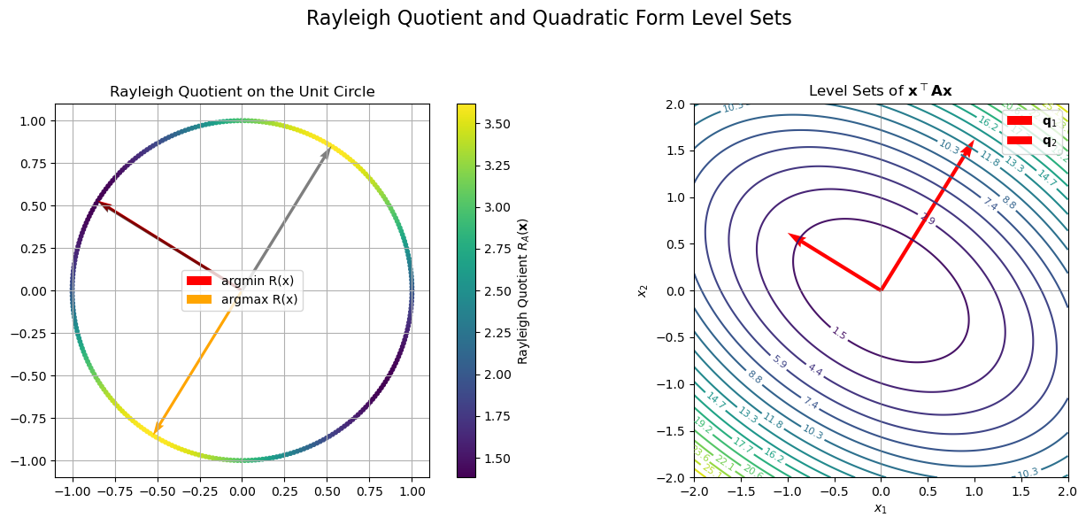
This combined visualization brings together the Rayleigh quotient and the level sets of the quadratic form \(\mathbf{x}^\top \mathbf{A} \mathbf{x}\):
Left panel: Rayleigh quotient \(R_\mathbf{A}(\mathbf{x})\) on the unit circle
Color shows how the value varies with direction.
Extremes occur at eigenvector directions (marked with arrows).
Right panel: Level sets (contours) of the quadratic form
Elliptical shapes aligned with eigenvectors.
Red vectors indicate principal axes (scaled eigenvectors).
Together, these panels illustrate how the direction of a vector determines how strongly it is scaled by the symmetric matrix, and how this scaling relates to the matrix’s eigenstructure.
✅ As guaranteed by the Min–Max Theorem, the maximum and minimum of the Rayleigh quotient occur precisely at the eigenvectors corresponding to the largest and smallest eigenvalues.