The fundamental subspaces of a matrix#
The fundamental subspaces of a matrix \(\mathbf{A}\) are the four subspaces associated with the matrix and its transpose. These subspaces are important in linear algebra and numerical analysis, particularly in the context of solving linear systems and eigenvalue problems.
We also provide the projections onto these subspaces, which are useful for various applications such as least squares problems and dimensionality reduction. The proof of these projection formulas relies on the properties of the Moore-Penrose pseudoinverse and the orthogonal projections onto subspaces.
We denote the matrix \(\mathbf{A}\) as an \(m \times n\) matrix, where \(m\) is the number of rows and \(n\) is the number of columns.
The four fundamental subspaces are:
Column Space (Range) of \(\mathbf{A}\):#
The column space of a matrix \(\mathbf{A}\) is the set of all possible linear combinations of its columns. It represents the span of the columns of \(\mathbf{A}\) and is denoted as \(\text{Col}(\mathbf{A})\) or \(\text{Range}(\mathbf{A})\). Intuitively, the column space is the set of all vectors \(\mathbf{b}_{\text{Col}}\) that you can reach by taking weighted sums of the columns of \(\mathbf{A},\) or the set of all vectors that produce a solvable linear equation system \(\mathbf{A}\mathbf{x}=\mathbf{b}_{\text{Col}}\).
Lemma (Projection onto the Column Space)
The projection of a vector \(\mathbf{b}\in\mathbb{R}^m\) onto the column space of a matrix \(\mathbf{A}\) is given by:
Proof. Let \(\mathbf{A} \in \mathbb{R}^{m \times n}\) and \(\mathbf{b} \in \mathbb{R}^m\). The Moore-Penrose pseudoinverse \(\mathbf{A}^+\) satisfies the property that \(\mathbf{A}\mathbf{A}^+\mathbf{A} = \mathbf{A}\) and \(\mathbf{A}^+\mathbf{A}\mathbf{A}^+ = \mathbf{A}^+\).
The vector \(\mathbf{A}\mathbf{A}^+\mathbf{b}\) is in the column space of \(\mathbf{A}\) because it is a linear combination of the columns of \(\mathbf{A}\).
We claim that \(\mathbf{A}\mathbf{A}^+\mathbf{b}\) is the unique vector in \(\text{Col}(\mathbf{A})\) closest to \(\mathbf{b}\) (i.e., the orthogonal projection).
To see this, recall that the orthogonal projection \(\mathbf{p}\) of \(\mathbf{b}\) onto \(\text{Col}(\mathbf{A})\) is the unique vector in \(\text{Col}(\mathbf{A})\) such that \(\mathbf{b} - \mathbf{p}\) is orthogonal to \(\text{Col}(\mathbf{A})\).
That is,
Let \(\mathbf{p} = \mathbf{A}\mathbf{x}\) for some \(\mathbf{x} \in \mathbb{R}^n\).
Then
If \(\mathbf{A}\) has full column rank, the solution is \(\mathbf{x} = (\mathbf{A}^\top \mathbf{A})^{-1} \mathbf{A}^\top \mathbf{b}\), so \(\mathbf{p} = \mathbf{A}(\mathbf{A}^\top \mathbf{A})^{-1} \mathbf{A}^\top \mathbf{b}\). For arbitrary \(\mathbf{A}\), the unique minimum-norm solution is \(\mathbf{x} = \mathbf{A}^+ \mathbf{b}\), so \(\mathbf{p} = \mathbf{A}\mathbf{A}^+ \mathbf{b}\).
Therefore, \(\mathbf{A}\mathbf{A}^+\mathbf{b}\) is the orthogonal projection of \(\mathbf{b}\) onto \(\text{Col}(\mathbf{A})\).
Row Space of \(\mathbf{A}\):#
The row space of a matrix \(\mathbf{A}\) is the set of all possible linear combinations of its rows.
It is equivalent to the column space of its transpose, \(\mathbf{A}^\top\), and is denoted as \(\text{Row}(\mathbf{A})\) or \(\text{Col}(\mathbf{A}^\top)\).
Intuitively, the row space consists of all vectors you can reach by taking weighted sums of the rows of \(\mathbf{A}\).
Lemma (Projection onto the Row Space)
The projection of a vector \(\mathbf{x}\in\mathbb{R}^n\) onto the row space of a matrix \(\mathbf{A}\) is given by:
Proof. Let \(\mathbf{A} \in \mathbb{R}^{m \times n}\) and \(\mathbf{x} \in \mathbb{R}^n\).
The row space of \(\mathbf{A}\) is the column space of \(\mathbf{A}^\top\).
Recall that the orthogonal projection of \(\mathbf{x}\) onto the row space of \(\mathbf{A}\) is the unique vector \(\mathbf{p}\) in \(\text{Row}(\mathbf{A})\) such that \(\mathbf{x} - \mathbf{p}\) is orthogonal to the row space.
That is, for all \(\mathbf{y}\) in the row space, \(\langle \mathbf{x} - \mathbf{p}, \mathbf{y} \rangle = 0\).
Let \(\mathbf{p} = \mathbf{A}^+\mathbf{A}\mathbf{x}\).
We want to show that \(\mathbf{x} - \mathbf{p}\) is orthogonal to the row space of \(\mathbf{A}\).
Any vector in the row space can be written as \(\mathbf{A}^\top \mathbf{w}\) for some \(\mathbf{w} \in \mathbb{R}^m\). Then,
since \(\mathbf{A}\mathbf{A}^+\mathbf{A} = \mathbf{A}\).
Thus, \(\mathbf{x} - \mathbf{A}^+\mathbf{A}\mathbf{x}\) is orthogonal to the row space, so \(\mathbf{A}^+\mathbf{A}\mathbf{x}\) is the orthogonal projection of \(\mathbf{x}\) onto the row space of \(\mathbf{A}\).
Furthermore, for any \(\mathbf{r}\) in the row space, \(\mathbf{r} = \mathbf{A}^\top \mathbf{w}\) for some \(\mathbf{w}\), and \(\mathbf{A}^+\mathbf{A}\mathbf{r} = \mathbf{A}^+\mathbf{A}\mathbf{A}^\top \mathbf{w} = \mathbf{A}^+\mathbf{A}\mathbf{A}^\top \mathbf{w} = \mathbf{r}\) (since \(\mathbf{A}^+\mathbf{A}\) acts as the identity on the row space). Thus, the operator acts as the identity on the row space.
Therefore, \(\mathbf{P}_{\text{Row}(\mathbf{A})} = \mathbf{A}^+\mathbf{A}\) is the orthogonal projection onto the row space of \(\mathbf{A}\).
Null Space (Kernel) of \(\mathbf{A}\):#
The null space of a matrix \(\mathbf{A}\) is the set of all vectors \(\mathbf{n}\in\mathbb{R}^n\) such that \(\mathbf{A}\mathbf{n} = \mathbf{0}\).
It represents the solutions to the homogeneous equation associated with \(\mathbf{A}\) and is denoted as \(\text{Null}(\mathbf{A})\) or \(\text{Ker}(\mathbf{A})\).
Intuitively, the null space consists of all input vectors that are “annihilated” by \(\mathbf{A}\), meaning they are mapped to the zero vector.
Lemma (Projection onto the Null Space)
The projection of a vector \(\mathbf{x}\in\mathbb{R}^n\) onto the null space of a matrix \(\mathbf{A}\) is given by:
Proof. Let \(\mathbf{A} \in \mathbb{R}^{m \times n}\) and \(\mathbf{x} \in \mathbb{R}^n\).
The null space of \(\mathbf{A}\) is the orthogonal complement of the row space of \(\mathbf{A}\), and the column space of \(\mathbf{A}\) is the orthogonal complement of the null space of \(\mathbf{A}^\top\).
Recall that the orthogonal projection of \(\mathbf{x}\) onto the row space of \(\mathbf{A}\) is \(\mathbf{A}^+\mathbf{A}\mathbf{x}\).
The projection onto the orthogonal complement (i.e., the null space) is then given by subtracting this projection from \(\mathbf{b}\):
To see that this is indeed a projection onto the null space, note that for any \(\mathbf{x}\), \(\mathbf{A}(\mathbf{x} - \mathbf{A}^+\mathbf{A}\mathbf{x}) = \mathbf{A}\mathbf{x} - \mathbf{A}\mathbf{A}^+\mathbf{A}\mathbf{x} = \mathbf{A}\mathbf{x} - \mathbf{A}\mathbf{x} = 0\), since \(\mathbf{A}\mathbf{A}^+\mathbf{A} = \mathbf{A}\).
Thus, \(\mathbf{x} - \mathbf{A}^+\mathbf{A}\mathbf{x}\) is in the null space of \(\mathbf{A}\).
Furthermore, for any \(\mathbf{n}\) in the null space of \(\mathbf{A}\), \(\mathbf{A}\mathbf{n} = 0\), so \(\mathbf{A}^+\mathbf{A}\mathbf{n} = 0\).
Thus, \(\mathbf{P}_{\text{Null}(\mathbf{A})}(\mathbf{n}) = \mathbf{n} - 0 = \mathbf{n}\), so the operator acts as the identity on the null space.
Therefore, \(\mathbf{P}_{\text{Null}(\mathbf{A})} = \mathbf{I} - \mathbf{A}^+\mathbf{A}\) is the orthogonal projection onto the null space of \(\mathbf{A}\).
Left Null Space of \(\mathbf{A}\):#
The left null space of a matrix \(\mathbf{A}\) is the set of all vectors \(\mathbf{y}\) such that \(\mathbf{A}^\top\mathbf{y} = \mathbf{0}\).
It represents the solutions to the homogeneous equation associated with \(\mathbf{A}^\top\) and is denoted as \(\text{Null}(\mathbf{A}^\top)\) or \(\text{Ker}(\mathbf{A}^\top)\). Intuitively, the left null space consists of all vectors that are orthogonal to every row of \(\mathbf{A}\), meaning they are “killed” by the transpose of \(\mathbf{A}\).
Lemma (Projection onto the Left Null Space)
The projection of a vector \(\mathbf{b}\) onto the left null space of a matrix \(\mathbf{A}\) is given by:
The proof is analogous to the one for the previous one.
Singular Value Decomposition and the four fundamental subspaces#
The Singular Value Decomposition (SVD) provides a powerful way to understand the four fundamental subspaces of a matrix \(\mathbf{A} \in \mathbb{R}^{m \times n}\) because it expresses \(\mathbf{A}\) in terms of orthogonal bases that directly reveal the structure of these subspaces. Intuitively, the SVD rotates and scales the input space so that the action of \(\mathbf{A}\) becomes transparent: the nonzero singular values indicate directions (and their magnitudes) along which \(\mathbf{A}\) stretches or compresses, while the zero singular values correspond to directions that are “flattened” to zero. The columns of the SVD matrices \(\mathbf{U}\) and \(\mathbf{V}\) thus provide natural bases for the column space, row space, null space, and left null space, making the relationships between these subspaces explicit.
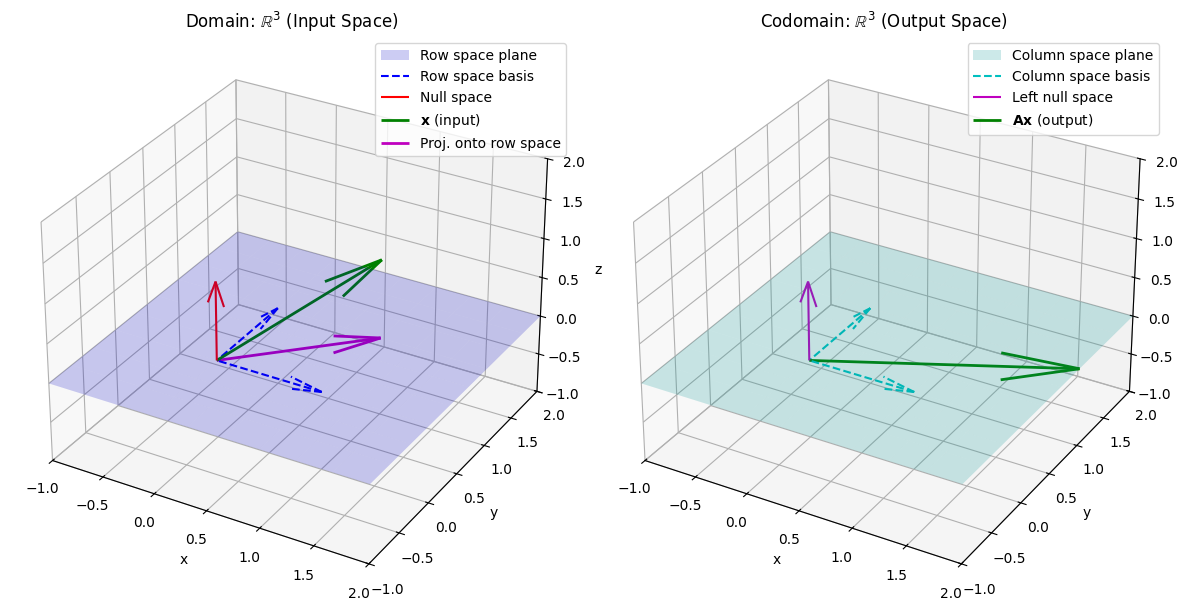
Python Visualization Example
Below is a visual demonstration of how the SVD of a \(3 \times 3\) matrix reveals its fundamental subspaces. We show how a vector is transformed by \(\mathbf{A}\), and how the SVD components relate to the column space, row space, and null space.
The Matrix \(\mathbf{A}\) and Vector \(\mathbf{x}\) used in the visualization are:
Show code cell source
import numpy as np
import matplotlib.pyplot as plt
from mpl_toolkits.mplot3d import Axes3D

# Define a 3x3 matrix of rank 2
A = np.array([[2, 0, 0],
              [0, 1, 0],
              [0, 0, 0]])

U, S, Vt = np.linalg.svd(A)
V = Vt.T

# Column space: span of first 2 columns of U
col_space = U[:, :2]
# Left null space: last column of U
left_null_space = U[:, 2:3]

# Row space: span of first 2 columns of V
row_space = V[:, :2]
# Null space: last column of V
null_space = V[:, 2:3]

fig = plt.figure(figsize=(12, 6))

# --- Domain (input space) ---
ax1 = fig.add_subplot(121, projection='3d')
ax1.set_title("Domain: $\\mathbb{R}^3$ (Input Space)")
ax1.set_xlim([-1, 2])
ax1.set_ylim([-1, 2])
ax1.set_zlim([-1, 2])

# Plot row space (plane)
# Create a grid of points for the plane
v1, v2 = row_space[:, 0], row_space[:, 1]
grid_x = np.linspace(-1, 2, 10)
grid_y = np.linspace(-1, 2, 10)
xx, yy = np.meshgrid(grid_x, grid_y)
plane_points = np.outer(v1, xx.flatten()) + np.outer(v2, yy.flatten())
plane_x = plane_points[0].reshape(xx.shape)
plane_y = plane_points[1].reshape(yy.shape)
plane_z = plane_points[2].reshape(xx.shape)
ax1.plot_surface(plane_x, plane_y, plane_z, color='b', alpha=0.2, label='Row space plane')

# Plot row space basis vectors
for v in row_space.T:
    ax1.quiver(0, 0, 0, v[0], v[1], v[2], color='b', linestyle='dashed', label='Row space basis' if 'Row space basis' not in ax1.get_legend_handles_labels()[1] else "")
# Plot null space
ax1.quiver(0, 0, 0, null_space[0,0], null_space[1,0], null_space[2,0], color='r', label='Null space')

# Example vector in domain
x = np.array([1, 1, 1])
ax1.quiver(0, 0, 0, x[0], x[1], x[2], color='g', label='$\\mathbf{x}$ (input)', linewidth=2)

# Projection of x onto the row space
# The projection is V_r V_r^T x, where V_r are the first two columns of V
V_r = row_space
x_row_proj = V_r @ (V_r.T @ x)
ax1.quiver(0, 0, 0, x_row_proj[0], x_row_proj[1], x_row_proj[2], color='m', label='Proj. onto row space', linewidth=2)

ax1.legend()
ax1.set_xlabel('x')
ax1.set_ylabel('y')
ax1.set_zlabel('z')

# --- Codomain (output space) ---
ax2 = fig.add_subplot(122, projection='3d')
ax2.set_title("Codomain: $\\mathbb{R}^3$ (Output Space)")
ax2.set_xlim([-1, 2])
ax2.set_ylim([-1, 2])
ax2.set_zlim([-1, 2])

# Plot column space (plane)
# Create a grid of points for the plane
u1, u2 = col_space[:, 0], col_space[:, 1]
grid_x2 = np.linspace(-1, 2, 10)
grid_y2 = np.linspace(-1, 2, 10)
xx2, yy2 = np.meshgrid(grid_x2, grid_y2)
plane_points2 = np.outer(u1, xx2.flatten()) + np.outer(u2, yy2.flatten())
plane_x2 = plane_points2[0].reshape(xx2.shape)
plane_y2 = plane_points2[1].reshape(yy2.shape)
plane_z2 = plane_points2[2].reshape(xx2.shape)
ax2.plot_surface(plane_x2, plane_y2, plane_z2, color='c', alpha=0.2, label='Column space plane')

# Plot column space basis vectors
for u in col_space.T:
    ax2.quiver(0, 0, 0, u[0], u[1], u[2], color='c', linestyle='dashed', label='Column space basis' if 'Column space basis' not in ax2.get_legend_handles_labels()[1] else "")
# Plot left null space
ax2.quiver(0, 0, 0, left_null_space[0,0], left_null_space[1,0], left_null_space[2,0], color='m', label='Left null space')

# Show image of x under A
Ax = A @ x
ax2.quiver(0, 0, 0, Ax[0], Ax[1], Ax[2], color='g', label='$\\mathbf{A}\\mathbf{x}$ (output)', linewidth=2)

ax2.legend()
ax2.set_xlabel('x')
ax2.set_ylabel('y')
ax2.set_zlabel('z')

plt.tight_layout()
plt.show()
Let the SVD of \(\mathbf{A}\) be:
where \(\mathbf{U} \in \mathbb{R}^{m \times m}\) and \(\mathbf{V} \in \mathbb{R}^{n \times n}\) are orthogonal matrices, and \(\mathbf{\Sigma} \in \mathbb{R}^{m \times n}\) is a diagonal matrix with the singular values of \(\mathbf{A}\) on its diagonal.
Lemma (SVD and the Four Fundamental Subspaces)
The SVD of a matrix \(\mathbf{A} \in \mathbb{R}^{m \times n}\) can be used to identify the four fundamental subspaces as follows:
Column Space: \(\text{Col}(\mathbf{A}) = \text{span}(\mathbf{U}_r)\), where \(\mathbf{U}_r\) consists of the first \(r\) columns of \(\mathbf{U}\) corresponding to non-zero singular values.
Row Space: \(\text{Row}(\mathbf{A}) = \text{span}(\mathbf{V}_r)\), where \(\mathbf{V}_r\) consists of the first \(r\) columns of \(\mathbf{V}\) corresponding to non-zero singular values.
Null Space: \(\text{Null}(\mathbf{A}) = \text{span}(\mathbf{V}_{n-r})\), where \(\mathbf{V}_{n-r}\) consists of the last \(n-r\) columns of \(\mathbf{V}\) corresponding to zero singular values.
Left Null Space: \(\text{Null}(\mathbf{A}^\top) = \text{span}(\mathbf{U}_{m-r})\), where \(\mathbf{U}_{m-r}\) consists of the last \(m-r\) columns of \(\mathbf{U}\) corresponding to zero singular values.
Proof. Let \(\mathbf{A} \in \mathbb{R}^{m \times n}\) have the singular value decomposition (SVD)
where \(\mathbf{U} \in \mathbb{R}^{m \times m}\) and \(\mathbf{V} \in \mathbb{R}^{n \times n}\) are orthogonal matrices, and \(\mathbf{\Sigma} \in \mathbb{R}^{m \times n}\) is diagonal with non-negative entries (the singular values) on the diagonal.
Suppose \(\mathbf{A}\) has rank \(r\), so that the first \(r\) singular values \(\sigma_1, \ldots, \sigma_r\) are positive, and the rest are zero. We can write
where \(\mathbf{D}_r = \operatorname{diag}(\sigma_1, \ldots, \sigma_r)\) is \(r \times r\).
Let \(\mathbf{U}_r\) denote the first \(r\) columns of \(\mathbf{U}\), and \(\mathbf{U}_{m-r}\) the last \(m-r\) columns. Similarly, let \(\mathbf{V}_r\) denote the first \(r\) columns of \(\mathbf{V}\), and \(\mathbf{V}_{n-r}\) the last \(n-r\) columns.
1. Column Space:
\(\mathbf{A} = \mathbf{U}_r \mathbf{D}_r \mathbf{V}_r^\top\) (since the rest of the singular values are zero). Thus, the columns of \(\mathbf{A}\) are linear combinations of the columns of \(\mathbf{U}_r\). Therefore,
2. Row Space:
The row space of \(\mathbf{A}\) is the column space of \(\mathbf{A}^\top\). The SVD of \(\mathbf{A}^\top\) is \(\mathbf{A}^\top = \mathbf{V} \mathbf{\Sigma}^\top \mathbf{U}^\top\). By the same reasoning as above, the row space is
3. Null Space:
A vector \(\mathbf{x} \in \mathbb{R}^n\) is in the null space of \(\mathbf{A}\) if \(\mathbf{A}\mathbf{x} = \mathbf{0}\). Write \(\mathbf{x}\) in the basis of \(\mathbf{V}\): \(\mathbf{x} = \mathbf{V} \mathbf{y}\) for some \(\mathbf{y} \in \mathbb{R}^n\). Then
This is zero if and only if the first \(r\) entries of \(\mathbf{y}\) are zero (since the corresponding singular values are nonzero), i.e., \(\mathbf{y} = \begin{bmatrix} 0 \\ \mathbf{y}_2 \end{bmatrix}\) where \(\mathbf{y}_2 \in \mathbb{R}^{n-r}\). Thus, the null space is spanned by the last \(n-r\) columns of \(\mathbf{V}\):
4. Left Null Space:
A vector \(\mathbf{y} \in \mathbb{R}^m\) is in the left null space if \(\mathbf{A}^\top \mathbf{y} = \mathbf{0}\). Write \(\mathbf{y} = \mathbf{U} \mathbf{z}\) for some \(\mathbf{z} \in \mathbb{R}^m\). Then
This is zero if and only if the first \(r\) entries of \(\mathbf{z}\) are zero (since the corresponding singular values are nonzero), i.e., \(\mathbf{z} = \begin{bmatrix} 0 \\ \mathbf{z}_2 \end{bmatrix}\) where \(\mathbf{z}_2 \in \mathbb{R}^{m-r}\). Thus, the left null space is spanned by the last \(m-r\) columns of \(\mathbf{U}\):
Summary#
The four fundamental subspaces of a matrix \(\mathbf{A}\) are essential in understanding the structure of the matrix and its properties. The projections onto these subspaces can be computed using the Moore-Penrose pseudoinverse, which provides a powerful tool for solving linear systems and performing dimensionality reduction. The SVD further enhances our understanding by revealing the relationships between these subspaces through the orthogonal matrices and singular values.