Orthogonal projections

We now consider a particular kind of optimization problem referred to as projection onto a subspace:

Given some point \(\mathbf{x}\) in an inner product space \(V\), find the closest point to \(\mathbf{x}\) in a subspace \(S\) of \(V\).

The following diagram should make it geometrically clear that, at least in Euclidean space, the solution is intimately related to orthogonality and the Pythagorean theorem:

Show code cell source Hide code cell source

# Re-import required packages due to kernel reset
import numpy as np
import matplotlib.pyplot as plt

# Define subspace S spanned by vector e1
e1 = np.array([1, 2])
e1 = e1 / np.linalg.norm(e1)  # normalize to make it orthonormal

# Define arbitrary point x not in the subspace
x = np.array([2, 1])

# Compute projection of x onto the subspace spanned by e1
x_proj = np.dot(x, e1) * e1

# Define a second point y in the subspace (for triangle)
y = 3 * e1

# Set up plot
fig, ax = plt.subplots(figsize=(6, 6))

# Draw vectors
origin = np.array([0, 0])
ax.quiver(*origin, *x, angles='xy', scale_units='xy', scale=1, color='blue', label=r'$\mathbf{x}$')
ax.quiver(*origin, *x_proj, angles='xy', scale_units='xy', scale=1, color='green', label=r'$\mathbf{y}^* = P\mathbf{x}$')
ax.quiver(*origin, *y, angles='xy', scale_units='xy', scale=1, color='gray', alpha=0.5, label=r'$\mathbf{y} \in S$')

# Draw dashed lines to form triangle
ax.plot([x[0], x_proj[0]], [x[1], x_proj[1]], 'k--', lw=1)
ax.plot([y[0], x[0]], [y[1], x[1]], 'k--', lw=1)
ax.plot([y[0], x_proj[0]], [y[1], x_proj[1]], 'k--', lw=1)

# Annotate
ax.text(*(x + 0.2), r'$\mathbf{x}$', fontsize=12)
ax.text(*(x_proj + 0.2), r'$\mathbf{y}^*$', fontsize=12)
ax.text(*(y + 0.2), r'$\mathbf{y}$', fontsize=12)

# Draw subspace line
line_extent = np.linspace(-10, 10, 100)
s_line = np.outer(line_extent, e1)
ax.plot(s_line[:, 0], s_line[:, 1], 'r-', lw=1, label=r'Subspace $S$')

# Formatting
ax.set_xlim(-0.5, 3)
ax.set_ylim(-0.5, 3)
ax.set_aspect('equal')
ax.grid(True)
ax.legend()
ax.set_title(r"Orthogonal Projection of $\mathbf{x}$ onto Subspace $S$")

plt.tight_layout()
plt.show()

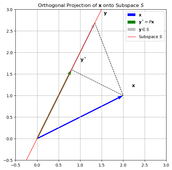
In this diagram, the blue vector \(\mathbf{x}\) is an arbitrary point in the inner product space \(V\), the green vector \(\mathbf{y}^* = \mathbf{P}\mathbf{x}\) is the projection of \(\mathbf{x}\) onto the subspace \(S\), and the gray vector \(\mathbf{y}\) is an arbitrary point in \(S\).

The dashed lines form a right triangle with \(\mathbf{x}\), \(\mathbf{y}^*\), and \(\mathbf{y}\) as vertices. The right triangle formed by these three points illustrates the relationship between the projection and orthogonality: the line segment from \(\mathbf{x}\) to \(\mathbf{y}^*\) is perpendicular to the subspace \(S\), and the distance from \(\mathbf{x}\) to \(\mathbf{y}^*\) is the shortest distance from \(\mathbf{x}\) to any point in \(S\).

This is a direct consequence of the Pythagorean theorem, which states that in a right triangle, the square of the length of the hypotenuse (in this case, \(\|\mathbf{x}-\mathbf{y}\|\)) is equal to the sum of the squares of the lengths of the other two sides (in this case, \(\|\mathbf{x}-\mathbf{y}^*\|\) and \(\|\mathbf{y}^*-\mathbf{y}\|\)).

Here \(\mathbf{y}\) is an arbitrary element of the subspace \(S\), and \(\mathbf{y}^*\) is the point in \(S\) such that \(\mathbf{x}-\mathbf{y}^*\) is perpendicular to \(S\). The hypotenuse of a right triangle (in this case \(\|\mathbf{x}-\mathbf{y}\|\)) is always longer than either of the legs (in this case \(\|\mathbf{x}-\mathbf{y}^*\|\) and \(\|\mathbf{y}^*-\mathbf{y}\|\)), and when \(\mathbf{y} \neq \mathbf{y}^*\) there always exists such a triangle between \(\mathbf{x}\), \(\mathbf{y}\), and \(\mathbf{y}^*\).

Our intuition from Euclidean space suggests that the closest point to \(\mathbf{x}\) in \(S\) has the perpendicularity property described above, and we now show that this is indeed the case.

Proposition (Ortogonal projection and unique minimizer)

Let \(S\) be a subspace of an inner product space \(V\) and let \(\mathbf{x} \in V\) and \(\mathbf{y} \in S\).

Then \(\mathbf{y}^*\) is the unique minimizer of \(\|\mathbf{x}-\mathbf{y}\|\) over \(\mathbf{y} \in S\) if and only if \(\mathbf{x}-\mathbf{y}^* \perp S\).

Proof. \((\implies)\) Suppose \(\mathbf{y}^*\) is the unique minimizer of \(\|\mathbf{x}-\mathbf{y}\|\) over \(\mathbf{y} \in S\).

That is, \(\|\mathbf{x}-\mathbf{y}^*\| \leq \|\mathbf{x}-\mathbf{y}\|\) for all \(\mathbf{y} \in S\), with equality only if \(\mathbf{y} = \mathbf{y}^*\).

Fix \(\mathbf{v} \in S\) and observe that

\[\begin{split}\begin{aligned} g(t) :&= \|\mathbf{x}-\mathbf{y}^*+t\mathbf{v}\|^2 \\ &= \langle \mathbf{x}-\mathbf{y}^*+t\mathbf{v}, \mathbf{x}-\mathbf{y}^*+t\mathbf{v} \rangle \\ &= \langle \mathbf{x}-\mathbf{y}^*, \mathbf{x}-\mathbf{y}^* \rangle - 2t\langle \mathbf{x}-\mathbf{y}^*, \mathbf{v} \rangle + t^2\langle \mathbf{v}, \mathbf{v} \rangle \\ &= \|\mathbf{x}-\mathbf{y}^*\|^2 - 2t\langle \mathbf{x}-\mathbf{y}^*, \mathbf{v} \rangle + t^2\|\mathbf{v}\|^2 \end{aligned}\end{split}\]

must have a minimum at \(t = 0\) as a consequence of this assumption.

Thus

\[0 = g'(0) = \left.-2\langle \mathbf{x}-\mathbf{y}^*, \mathbf{v} \rangle + 2t\|\mathbf{v}\|^2\right|_{t=0} = -2\langle \mathbf{x}-\mathbf{y}^*, \mathbf{v} \rangle\]

giving \(\mathbf{x}-\mathbf{y}^* \perp \mathbf{v}\). Since \(\mathbf{v}\) was arbitrary in \(S\), we have \(\mathbf{x}-\mathbf{y}^* \perp S\) as claimed.

\((\impliedby)\) Suppose \(\mathbf{x}-\mathbf{y}^* \perp S\).

Observe that for any \(\mathbf{y} \in S\), \(\mathbf{y}^*-\mathbf{y} \in S\) because \(\mathbf{y}^* \in S\) and \(S\) is closed under subtraction.

Under the hypothesis, \(\mathbf{x}-\mathbf{y}^* \perp \mathbf{y}^*-\mathbf{y}\), so by the Pythagorean theorem,

\[\|\mathbf{x}-\mathbf{y}\| = \|\mathbf{x}-\mathbf{y}^*+\mathbf{y}^*-\mathbf{y}\| = \|\mathbf{x}-\mathbf{y}^*\| + \|\mathbf{y}^*-\mathbf{y}\| \geq \|\mathbf{x} - \mathbf{y}^*\|\]

and in fact the inequality is strict when \(\mathbf{y} \neq \mathbf{y}^*\) since this implies \(\|\mathbf{y}^*-\mathbf{y}\| > 0\).

Thus \(\mathbf{y}^*\) is the unique minimizer of \(\|\mathbf{x}-\mathbf{y}\|\) over \(\mathbf{y} \in S\). ◻

Since a unique minimizer in \(S\) can be found for any \(\mathbf{x} \in V\), we can define an operator

\[\mathbf{P}\mathbf{x} = \operatorname{argmin}_{\mathbf{y} \in S} \|\mathbf{x}-\mathbf{y}\|\]

Observe that \(\mathbf{P}\mathbf{y} = \mathbf{y}\) for any \(\mathbf{y} \in S\), since \(\mathbf{y}\) has distance zero from itself and every other point in \(S\) has positive distance from \(\mathbf{y}\).

Thus \(\mathbf{\mathbf{P}}(\mathbf{\mathbf{P}}\mathbf{x}) = \mathbf{P}\mathbf{x}\) for any \(\mathbf{x}\) (i.e., \(\mathbf{P}^2 = \mathbf{P}\)) because \(\mathbf{P}\mathbf{x} \in S\).

The identity \(\mathbf{P}^2 = \mathbf{P}\) is actually one of the defining properties of a projection, the other being linearity.

An immediate consequence of the previous result is that \(\mathbf{x} - \mathbf{P}\mathbf{x} \perp S\) for any \(\mathbf{x} \in V\), and conversely that \(\mathbf{P}\) is the unique operator that satisfies this property for all \(\mathbf{x} \in V\). For this reason, \(\mathbf{P}\) is known as an orthogonal projection.

If we choose an orthonormal basis for the target subspace \(S\), it is possible to write down a more specific expression for \(\mathbf{P}\).

Proposition

If \(\mathbf{e}_1, \dots, \mathbf{e}_m\) is an orthonormal basis for \(S\), then

\[\mathbf{P}\mathbf{x} = \sum_{i=1}^m \langle \mathbf{x}, \mathbf{e}_i \rangle\mathbf{e}_i\]

Proof. Let \(\mathbf{e}_1, \dots, \mathbf{e}_m\) be an orthonormal basis for \(S\), and suppose \(\mathbf{x} \in V\).

Then for all \(j = 1, \dots, m\),

\[\begin{split}\begin{aligned} \left\langle \mathbf{x}-\sum_{i=1}^m \langle \mathbf{x}, \mathbf{e}_i \rangle\mathbf{e}_i, \mathbf{e}_j \right\rangle &= \langle \mathbf{x}, \mathbf{e}_j \rangle - \sum_{i=1}^m \langle \mathbf{x}, \mathbf{e}_i \rangle\underbrace{\langle \mathbf{e}_i, \mathbf{e}_j \rangle}_{\delta_{ij}} \\ &= \langle \mathbf{x}, \mathbf{e}_j \rangle - \langle \mathbf{x}, \mathbf{e}_j \rangle \\ &= 0 \end{aligned}\end{split}\]

We have shown that the claimed expression, call it \(\tilde{\mathbf{P}}\mathbf{x}\), satisfies \(\mathbf{x} - \tilde{\mathbf{P}}\mathbf{x} \perp \mathbf{e}_j\) for every element \(\mathbf{e}_j\) of the orthonormal basis for \(S\).

It follows (by linearity of the inner product) that \(\mathbf{x} - \tilde{\mathbf{P}}\mathbf{x} \perp S\).

So the previous result implies \(\mathbf{P} = \tilde{\mathbf{P}}\). ◻

The fact that \(\mathbf{P}\) is a linear operator (and thus a proper projection, as earlier we showed \(\mathbf{P}^2 = \mathbf{P}\)) follows readily from this result.

Matrix Representation of Projection Operators

Given a subspace \(S \subset \mathbb{R}^n\), the orthogonal projection of a vector \(\mathbf{x} \in \mathbb{R}^n\) onto \(S\) is the unique vector \(\mathbf{P}\mathbf{x} \in S\) such that:

• \(\mathbf{x} - \mathbf{P}\mathbf{x} \perp S\) (residual is orthogonal)

• \(\mathbf{P}\mathbf{x} \in S\) (lies in the subspace)

• \(\|\mathbf{x} - \mathbf{P}\mathbf{x}\|\) is minimized

This leads us to define the projection operator \(\mathbf{P} \in \mathbb{R}^{n \times n}\) as a linear map satisfying key properties — two of which are:

• idempotence \((\mathbf{P}^2 = \mathbf{P})\)

• symmetry \((\mathbf{P}^\top = \mathbf{P})\)

Let’s now examine why they are essential.

Idempotence \(\mathbf{P}^2 = \mathbf{P}\) is Required

Idempotence ensures that once you’ve projected a vector onto the subspace, projecting it again does nothing:

\[ \mathbf{P}(\mathbf{P}\mathbf{x}) = \mathbf{P}\mathbf{x} \]

Why it’s required:

• Geometrically: The image \(\mathbf{P}\mathbf{x}\) lies in the subspace. If projecting it again changed it, that would mean the subspace is not invariant under the projection — contradicting the notion of projection.

• Algebraically: If \(\mathbf{P}^2 \neq \mathbf{P}\), then \(\mathbf{P}\) is not consistent — it cannot define a fixed mapping to the subspace.

Why Symmetry \(\mathbf{P}^\top = \mathbf{P}\) is Required

Symmetry ensures that the projection is orthogonal: the difference between \(\mathbf{x}\) and its projection is orthogonal to the subspace:

\[ \langle \mathbf{x} - \mathbf{P}\mathbf{x}, \mathbf{P}\mathbf{x} \rangle = 0 \quad \Leftrightarrow \quad \mathbf{P}^\top = \mathbf{P} \]

Why it’s required:

• Without symmetry, \(\mathbf{P}\) could project onto the subspace in a skewed or oblique manner — not orthogonally.

• Orthogonal projections are characterized by minimal distance, and this only occurs when the residual is orthogonal to the subspace.

• If \(\mathbf{P} \neq \mathbf{P}^\top\), the projection may preserve direction, but not minimize distance.

Geometric Consequence:

A non-symmetric idempotent matrix defines an oblique projection, which is still a projection but not orthogonal. It does not minimize distance to the subspace.

Summary Table

Property	Meaning	Why Required
\(\mathbf{P}^2 = \mathbf{P}\)	Idempotence / Stability	Ensures projecting twice gives same result
\(\mathbf{P}^\top = \mathbf{P}\)	Symmetry / Orthogonality	Ensures projection is shortest-distance (orthogonal)

---

Basis Representation of Orthogonal Projection Matrices

Orthogonal projections can be expressed using matrices when the subspace is defined by a basis:

If \(S = \operatorname{span}(\mathbf{e}_1, \dots, \mathbf{e}_m)\), where the \(\mathbf{e}_i\) are orthonormal, then the projection matrix is:

\[ \mathbf{P} = \sum_{i=1}^m \mathbf{e}_i \mathbf{e}_i^\top \]

In matrix form, if \( E \in \mathbb{R}^{n \times m} \) has columns \(\mathbf{e}_i\), then

\[ \mathbf{P} = EE^\top \quad \text{and} \quad \mathbf{P}\mathbf{x} = EE^\top \mathbf{x} \]

Theorem (Basis Representation of the Orthogonal Projection Matrix)

Let \(\mathbf{e}_1, \dots, \mathbf{e}_m \in \mathbb{R}^n\) be orthonormal vectors, and define the matrix:

\[ E = [\mathbf{e}_1 \,\, \mathbf{e}_2 \,\, \cdots \,\, \mathbf{e}_m] \in \mathbb{R}^{n \times m} \]

Then the matrix:

\[ \mathbf{P} = EE^\top \in \mathbb{R}^{n \times n} \]

is the orthogonal projection onto the subspace \(S = \operatorname{Col}(E) = \operatorname{span}(\mathbf{e}_1, \dots, \mathbf{e}_m)\).

That is, for any \(\mathbf{x} \in \mathbb{R}^n\), \(\mathbf{P}\mathbf{x} \in S\), and \(\mathbf{x} - \mathbf{P}\mathbf{x} \perp S\).

Proof. Let’s verify the three key properties of orthogonal projections.

---

1. \(\mathbf{P}\) is symmetric:

\[ \mathbf{P}^\top = (EE^\top)^\top = EE^\top = \mathbf{P} \quad \text{✓} \]

---

2. \(\mathbf{P}\) is idempotent:

\[ \mathbf{P}^2 = (EE^\top)(EE^\top) = E(E^\top E)E^\top \]

But since \(\{\mathbf{e}_i\}\) are orthonormal, we have:

\[ E^\top E = I_m \Rightarrow \mathbf{P}^2 = E I E^\top = EE^\top = \mathbf{P} \quad \text{✓} \]

---

3. \(\mathbf{P}\mathbf{x} \in S\) and \(\mathbf{x} - \mathbf{P}\mathbf{x} \perp S\):

Let \(\mathbf{x} \in \mathbb{R}^n\). Then:

\[ \mathbf{P}\mathbf{x} = EE^\top \mathbf{x} \in \operatorname{Col}(E) = S \]

Let \(\mathbf{v} \in S\), so \(\mathbf{v} = E\mathbf{a}\) for some \(\mathbf{a} \in \mathbb{R}^m\). Then:

\[ \langle \mathbf{x} - \mathbf{P}\mathbf{x}, \mathbf{v} \rangle = \langle \mathbf{x} - EE^\top \mathbf{x}, E\mathbf{a} \rangle = \langle \mathbf{x}, E\mathbf{a} \rangle - \langle EE^\top \mathbf{x}, E\mathbf{a} \rangle \]

Use \(\langle \mathbf{x}, E\mathbf{a} \rangle = \langle E^\top \mathbf{x}, \mathbf{a} \rangle\), and similarly for the second term:

\[ = \langle E^\top \mathbf{x}, \mathbf{a} \rangle - \langle E^\top EE^\top \mathbf{x}, \mathbf{a} \rangle = \langle E^\top \mathbf{x}, \mathbf{a} \rangle - \langle E^\top \mathbf{x}, \mathbf{a} \rangle = 0 \]

So:

\[ \mathbf{x} - \mathbf{P}\mathbf{x} \perp S \quad \text{✓} \]

We conclude that \(\mathbf{P} = EE^\top = \sum_{i=1}^m \mathbf{e}_i \mathbf{e}_i^\top\) is indeed the orthogonal projection onto the subspace spanned by \(\{\mathbf{e}_1, \dots, \mathbf{e}_m\}\).

Application Example: Least Squares Regression

In least squares regression, we want to find the best-fitting line (or hyperplane) through a set of points.

This can be framed as an orthogonal projection problem:

Given a design matrix \(\mathbf{X} \in \mathbb{R}^{n \times d}\) and target vector \(\mathbf{y} \in \mathbb{R}^n\), the goal is to find coefficients \(\boldsymbol{\beta} \in \mathbb{R}^d\) such that: $\( \hat{\boldsymbol{\beta}} = \operatorname{argmin}_{\boldsymbol{\beta}} \|\mathbf{y} - \mathbf{X}\boldsymbol{\beta}\|^2 \)$

This is equivalent to projecting \(\mathbf{y}\) onto the column space of \(\mathbf{X}\), which can be expressed using the projection matrix:

\[ \mathbf{P} = \mathbf{X}(\mathbf{X}^\top \mathbf{X})^{-1}\mathbf{X}^\top = \mathbf{X}\mathbf{X}^+ \]

This projection minimizes the distance between \(\mathbf{y}\) and the subspace spanned by the columns of \(\mathbf{X}\), yielding the least squares solution.