Probability Basics#
Suppose we have some sort of randomized experiment (e.g. a coin toss, die roll) that has a fixed set of possible outcomes.
The set of possible outcomes of a random experiment is called the sample space and denoted
\[\Omega = \{ \text{all possible outcomes $\omega$ of the experiment} \}\]
An example of a sample space is the set of all possible outcomes of a coin toss:
Events are subsets of \(\Omega\) for which we want to assign probabilities.
For example, the event “the coin lands heads” is the subset \(\{ \text{heads} \}\) of \(\Omega\).
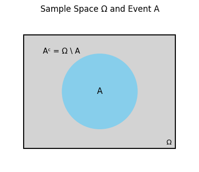
The complement of the event \(A\) is another event,
\[A^\text{c} = \Omega \setminus A.\]
For example, the complement of the event “the coin lands heads” is the event “the coin lands tails”, i.e. \(\{ \text{tails} \}\).
Below we visualize the sample space \(\Omega\), an event \(A\), and its complement \(A^\text{c}\):
Show code cell source
import matplotlib.pyplot as plt
import matplotlib.patches as patches

def plot_sample_space_and_event():
    fig, ax = plt.subplots(figsize=(6, 4))
    # Sample space Ω
    rect = patches.Rectangle((0, 0), 4, 3, linewidth=1.5, edgecolor='black', facecolor='lightgray')
    ax.add_patch(rect)
    # Event A
    circle = patches.Circle((2, 1.5), 1, facecolor='skyblue', edgecolor=None)
    ax.add_patch(circle)

    ax.text(3.75, 0.1, 'Ω', fontsize=10)
    ax.text(2, 1.5, 'A', fontsize=12, ha='center', va='center')
    ax.text(0.5, 2.5, 'Aᶜ = Ω \\ A', fontsize=11)
    ax.set_xlim(-0.5, 4.5)
    ax.set_ylim(-0.5, 3.5)
    ax.set_aspect('equal')
    ax.axis('off')
    plt.title('Sample Space Ω and Event A')
    plt.show()

def plot_event_and_complement():
    fig, ax = plt.subplots(figsize=(6, 4))
    rect = patches.Rectangle((0, 0), 4, 3, linewidth=1.5, edgecolor='black', facecolor='white')
    ax.add_patch(rect)
    ax.text(3.2, 2.5, 'Ω', fontsize=10)

    # Event A
    circle = patches.Circle((2, 1.5), 1, facecolor='skyblue', edgecolor='black')
    ax.add_patch(circle)
    ax.text(2, 1.5, 'A', fontsize=12, ha='center', va='center')

    # Label Aᶜ outside the circle but inside Ω
    ax.text(0.5, 2.5, 'Aᶜ = Ω \\ A', fontsize=11)

    ax.set_xlim(-0.5, 4.5)
    ax.set_ylim(-0.5, 3.5)
    ax.set_aspect('equal')
    ax.axis('off')
    plt.title('Event A and its Complement Aᶜ')
    plt.show()

def plot_disjoint_events():
    fig, ax = plt.subplots(figsize=(6, 4))
    rect = patches.Rectangle((0, 0), 5, 3.5, linewidth=1.5, edgecolor='black', facecolor='white')
    ax.add_patch(rect)

    circle1 = patches.Circle((1.5, 1.75), 1, facecolor='lightgreen', edgecolor='black')
    circle2 = patches.Circle((3.5, 1.75), 1, facecolor='orange', edgecolor='black')
    ax.add_patch(circle1)
    ax.add_patch(circle2)

    ax.text(1.5, 1.75, 'A₁', fontsize=12, ha='center', va='center')
    ax.text(3.5, 1.75, 'A₂', fontsize=12, ha='center', va='center')
    ax.text(3.7, 3.2, 'Ω', fontsize=10)

    ax.set_xlim(-0.5, 5.5)
    ax.set_ylim(-0.5, 4)
    ax.set_aspect('equal')
    ax.axis('off')
    plt.title('Disjoint Events A₁ and A₂ (A₁ ∩ A₂ = ∅)')
    plt.show()

def plot_probability_measure():
    events = ['A₁', 'A₂', 'A₃']
    probs = [0.2, 0.3, 0.1]

    plt.figure(figsize=(6, 4))
    bars = plt.bar(events, probs, color='mediumpurple')
    plt.ylim(0, 1.1)
    plt.axhline(1.0, color='gray', linestyle='--', label='P(Ω) = 1')
    plt.ylabel('Probability')
    plt.title('Probabilities of Disjoint Events: Countable Additivity')
    plt.legend()
    plt.show()


plot_sample_space_and_event()
# plot_event_and_complement()
#plot_disjoint_events()
#plot_probability_measure()
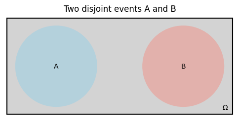
Two events \(A\) and \(B\) are disjoint if they have no outcomes in common, i.e. \(A \cap B = \varnothing\).
For example, the events “the coin lands heads” and “the coin lands tails” are disjoint.
Below, we visualize the sample space \(\Omega\), two disjoint events \(A\) and \(B\).
Show code cell source
import matplotlib.pyplot as plt
from matplotlib_venn import venn2, venn2_circles
import matplotlib.patches as patches

def plot_overlapping_events():
    # fig, ax = plt.figure(figsize=(6, 4))
    fig, ax = plt.subplots(figsize=(6, 4))
    rect = patches.Rectangle((-0.7, -0.47), 1.4, 0.94, linewidth=1.5, edgecolor='black', facecolor='lightgray')
    ax.add_patch(rect)
    ax.text(0.62, -0.44, 'Ω', fontsize=10)
    venn = venn2(subsets=(1, 1, 0.5), set_labels=('', ''),  set_colors=('skyblue', 'salmon')) # Ω is not shown
    venn.get_label_by_id('10').set_text('A')
    venn.get_label_by_id('01').set_text('B') # Aᶜ is not shown
    venn.get_label_by_id('11').set_text('A ∩ B') # ∅ is not shown
    plt.title('Two overlapping events A and B')
    plt.show()

def plot_disjoint_events():
    # plt.figure(figsize=(6, 4))
    fig, ax = plt.subplots(figsize=(6, 4))
    rect = patches.Rectangle((-1.1, -0.47), 2.2, 0.94, linewidth=1.5, edgecolor='black', facecolor='lightgray')
    ax.add_patch(rect)
    ax.text(1, -0.42, 'Ω', fontsize=10)
    venn = venn2(subsets=(1, 1, 0), set_labels=('', ''), set_colors=('skyblue', 'salmon'))
    venn.get_label_by_id('10').set_text('A')
    venn.get_label_by_id('01').set_text('B')
    plt.title('Two disjoint events A and B')
    plt.show()


def explain_probability_measure():
    events = ['A₁', 'A₂', 'A₃']
    probs = [0.2, 0.3, 0.1]
    plt.figure(figsize=(6, 4))
    plt.bar(events, probs, color='purple')
    plt.axhline(1.0, color='gray', linestyle='--', linewidth=0.8)
    plt.title('Probabilities of Disjoint Events (Add up to ≤ 1)')
    plt.ylabel('Probability')
    plt.show()

# plot_overlapping_events()
plot_disjoint_events()
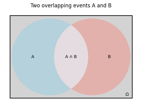
In comparison, below we visualize the sample space \(\Omega\), two overlapping events \(A\) and \(B\) and their intersection \(A \cap B\).
Show code cell source
plot_overlapping_events()
The set of possible events is denoted \(\mathcal{F}\).
(\(\mathcal{F}\) is a so-called \(\sigma\)-algebra of subsets of \(\Omega\).)
So \(\mathcal{F}\) is a set of sets of outcomes. We do not need to specify \(\mathcal{F}\) explicitly, but it is useful to know that it exists. Also the term \(\sigma\)-algebra is a bit technical and we will not use it in this course.
The goal of probability theory is to assign probabilities to events. To do so, we need to define a probability measure \(\mathbb{P} : \mathcal{F} \to [0,1]\) which must satisfy the following axioms:
Let \(\mathbb{P} : \mathcal{F} \to [0,1]\) be a probability measure which must satisfy
(i) \(\mathbb{P}(\Omega) = 1\)
(ii) Countable additivity: for any countable collection of disjoint sets \(\{A_i\} \subseteq \mathcal{F}\),
\[\mathbb{P}\bigg(\bigcup_i A_i\bigg) = \sum_i \mathbb{P}(A_i)\]
The triple \((\Omega, \mathcal{F}, \mathbb{P})\) is called a probability space.
If \(\mathbb{P}(A) = 1\), we say that \(A\) occurs almost surely (often abbreviated a.s.)., and conversely \(A\) occurs almost never if \(\mathbb{P}(A) = 0\).
From these axioms, a number of useful rules can be derived.
Proposition (Probability axioms)
Let \(A\) be an event.
Then
(i) \(\mathbb{P}(A^\text{c}) = 1 - \mathbb{P}(A)\).
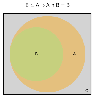
(ii) If \(B\) is an event and \(B \subseteq A\), then \(\mathbb{P}(B) \leq \mathbb{P}(A)\).
(iii) \(0 = \mathbb{P}(\varnothing) \leq \mathbb{P}(A) \leq \mathbb{P}(\Omega) = 1\)
To illustrate (ii) let’s plot a set \(A_1\) and its subset \(A_2\).
Show code cell source
def plot_subset_events():
    # plt.figure(figsize=(6, 4))
    fig, ax = plt.subplots(figsize=(6, 4))
    rect = patches.Rectangle((-0.6, -0.6), 1.3, 1.2, linewidth=1.5, edgecolor='black', facecolor='lightgray')
    ax.add_patch(rect)
    ax.text(0.62, -0.56, 'Ω', fontsize=10)
    venn = venn2(subsets=(0, 1, 1), set_labels=('', ''), set_colors=('green', 'orange'))
    venn.get_label_by_id('10').set_text('')
    venn.get_label_by_id('11').set_text('B')
    venn.get_label_by_id('01').set_text('A')
    plt.title('B ⊆ A ⇒ A ∩ B = B')
    plt.show()

plot_subset_events()
Proof. (i) Using the countable additivity of \(\mathbb{P}\), we have
To show (ii), suppose \(B \in \mathcal{F}\) and \(B \subseteq A\). Then
as claimed.
For (iii): the middle inequality follows from (ii) since \(\varnothing \subseteq A \subseteq \Omega\).
We also have
by countable additivity, which shows \(\mathbb{P}(\varnothing) = 0\).
Proposition
If \(A\) and \(B\) are events, then \(\mathbb{P}(A \cup B) = \mathbb{P}(A) + \mathbb{P}(B) - \mathbb{P}(A \cap B)\).
Proof. The key is to break the events up into their various overlapping and non-overlapping parts.
◻
Proposition (Union bound)
If \(\{A_i\} \subseteq \mathcal{F}\) is a countable set of events, disjoint or not, then
This inequality is sometimes referred to as Boole’s inequality or the union bound.
Proof. Define \(B_1 = A_1\) and \(B_i = A_i \setminus (\bigcup_{j < i} A_j)\) for \(i > 1\), noting that \(\bigcup_{j \leq i} B_j = \bigcup_{j \leq i} A_j\) for all \(i\) and the \(B_i\) are disjoint. Then
where the last inequality follows by monotonicity since \(B_i \subseteq A_i\) for all \(i\).
Conditional probability#
The conditional probability of event \(A\) given that event \(B\) has occurred is written \(\mathbb{P}(A | B)\) and defined as
assuming \(\mathbb{P}(B) > 0\).
Chain rule of probability#
Another very useful tool, the chain rule, follows immediately from this definition:
Bayes’ rule#
Taking the equality from above one step further, we arrive at the simple but crucial Bayes’ rule:
It is sometimes beneficial to omit the normalizing constant and write
Under this formulation, \(\mathbb{P}(A)\) is often referred to as the prior, \(\mathbb{P}(A | B)\) as the posterior, and \(\mathbb{P}(B | A)\) as the likelihood.
In the context of machine learning, we can use Bayes’ rule to update our “beliefs” (e.g. values of our model parameters) given some data that we’ve observed.