Principal Components Analysis#
Pricnipal Components Analysis (PCA) performs the orthogonal projection of the data onto a lower dimensional linear space. The goal is to find the directions (principal components) in which the variance of the data is maximized. An alternative definition of PCA is based on minimizing the sum-of-sqares of the projection errors.
Formal definition#
Given a dataset \(\mathbf{X} \in \mathbb{R}^{N \times D}\) (rows are samples, columns are features), we aim to find an orthonormal basis \(\mathbf{U}_k \in \mathbb{R}^{D \times k}\), \(k < D\), such that the projection of the data onto the subspace spanned by \(\mathbf{U}_k\) captures as much variance (energy) as possible.
In the following example, we visualize how PCA both minimizes reconstruction error in the original space and extracts a lower-dimensional, variance-preserving representation.
Show code cell source
import numpy as np
import pandas as pd
import matplotlib.pyplot as plt
from pysnptools.snpreader import Bed
from mpl_toolkits.mplot3d import Axes3D

# Generate synthetic 3D data
np.random.seed(42)
n_samples = 20
covariance_3d = np.array([
    [5, 0.5, 0.7],
    [0.5, 1, 0],
    [0.7, 0, 10]
])
rotation_3d = np.linalg.cholesky(covariance_3d)
data_3d = np.random.randn(n_samples, 3) @ rotation_3d.T

# Center the data
mean_3d = np.mean(data_3d, axis=0)
data_centered_3d = data_3d - mean_3d

# Compute SVD
U, S, Vt = np.linalg.svd(data_centered_3d, full_matrices=False)
V = Vt.T
S2 = S[:2] / np.sqrt(n_samples)
V2 = V[:, :2]

# Project and reconstruct
proj_2d = data_centered_3d @ V2
recon_3d = (proj_2d @ V2.T) + mean_3d[np.newaxis, :]

# Create a mesh grid for the 2D PCA plane
grid_range = np.linspace(-2, 2, 100)
xx, yy = np.meshgrid(grid_range, grid_range)
plane_points = np.stack([xx.ravel(), yy.ravel()], axis=1)
plane_points *= S2[np.newaxis, :]
plane_3d = mean_3d[np.newaxis, :] + (plane_points @ V2.T)

# Plot: 3D PCA + 2D Projection with principal components added in 2D view

fig = plt.figure(figsize=(16, 6))

# 3D plot
ax1 = fig.add_subplot(121, projection='3d')
ax1.scatter(data_3d[:, 0], data_3d[:, 1], data_3d[:, 2], alpha=0.2, label='Original Data')
ax1.scatter(recon_3d[:, 0], recon_3d[:, 1], recon_3d[:, 2], alpha=0.6, label='Projected (Reconstructed) Points')
for i in range(n_samples):
    ax1.plot(
        [data_3d[i, 0], recon_3d[i, 0]],
        [data_3d[i, 1], recon_3d[i, 1]],
        [data_3d[i, 2], recon_3d[i, 2]],
        'gray', lw=0.5, alpha=0.5
    )
ax1.plot_trisurf(plane_3d[:, 0], plane_3d[:, 1], plane_3d[:, 2], alpha=0.3, color='orange')
origin = mean_3d
ax1.quiver(*origin, *V[:, 0]*S2[0]*2, color='r', lw=2)
ax1.quiver(*origin, *V[:, 1]*S2[1]*2, color='blue', lw=2)

ax1.set_title("PCA in 3D: Projection onto First Two PCs")
ax1.set_xlabel("X")
ax1.set_ylabel("Y")
ax1.set_zlabel("Z")
ax1.legend()

# 2D projection plot
ax2 = fig.add_subplot(122)
ax2.scatter(proj_2d[:, 0], proj_2d[:, 1], alpha=0.8, c='orange', label='2D Projection')
# draw PC directions
ax2.plot([0, S2[0]*2], [0, 0], color='r', lw=2, label='1st PC')  # x-axis
ax2.plot([0, 0], [0, S2[1]*2], color='blue', lw=2, label='2nd PC')  # y-axis
ax2.axhline(0, color='gray', lw=0.5)
ax2.axvline(0, color='gray', lw=0.5)
ax2.set_title("Data Projected onto First Two Principal Components")
ax2.set_xlabel("1st PC")
ax2.set_ylabel("2nd PC")
ax2.axis('equal')
ax2.grid(True)
ax2.legend()

plt.tight_layout()
plt.show()
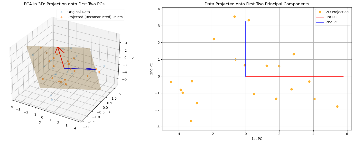
Left panel: The original 3D data, its projection onto the best-fit 2D PCA plane (orange), and reconstruction lines showing projection error.
Right panel: The same data projected onto the first two principal components, visualized in 2D.
Step 1: Center the Data#
We begin by centering the dataset so that the empirical mean is 0:
Define \(\mathbf{X} \leftarrow \mathbf{X}_{\text{centered}}\) for the rest of the derivation.
Step 2: Define the Projection#
Let \(\mathbf{U}_k \in \mathbb{R}^{D \times k}\) be an orthonormal matrix: \(\mathbf{U}_k^\top \mathbf{U}_k = \mathbf{I}_k\).
Project each sample \(\mathbf{x}_i \in \mathbb{R}^D\) onto the subspace:
The projection matrix is:
Step 3: Define the Reconstruction Error#
We want to minimize the total squared reconstruction error (projection error):
In matrix form:
where \(\|\cdot\|_F\) denotes the Frobenius norm.
Step 4: Reformulate as a Maximization Problem#
Instead of minimizing reconstruction error, we maximize the variance (energy) retained:
This comes from noting:
Step 5: Solve Using the Spectral Theorem#
Let \(\mathbf{X}^\top \mathbf{X} = \mathbf{M} \in \mathbb{R}^{D \times D}\). This matrix is symmetric and positive semidefinite.
By the spectral theorem, there exists an orthonormal basis of eigenvectors \(\mathbf{u}_1, \dots, \mathbf{u}_D\) with eigenvalues \(\lambda_1 \ge \lambda_2 \ge \dots \ge \lambda_D \ge 0\), such that:
Choose \(\mathbf{U}_k = [\mathbf{u}_1, \dots, \mathbf{u}_k]\) to maximize \(\text{tr}( \mathbf{U}_k^\top \mathbf{M} \mathbf{U}_k )\).
This is optimal because trace is maximized by choosing eigenvectors with largest eigenvalues (known from Rayleigh-Ritz and Courant-Fischer principles).
PCA Derivation Summary#
Input: Centered data matrix (\mathbf{X} \in \mathbb{R}^{N \times D})
Goal: Find orthonormal matrix (\mathbf{U}_k \in \mathbb{R}^{D \times k}) that captures most variance
Solution: Maximize ( \text{tr}(\mathbf{U}_k^\top \mathbf{X}^\top \mathbf{X} \mathbf{U}_k) ), subject to ( \mathbf{U}_k^\top \mathbf{U}_k = \mathbf{I} )
Optimal: Columns of (\mathbf{U}_k) are top (k) eigenvectors of ( \mathbf{X}^\top \mathbf{X} )
Projection: ( \mathbf{Z} = \mathbf{X} \mathbf{U}_k )
Reconstruction: ( \tilde{\mathbf{X}} = \mathbf{Z} \mathbf{U}_k^\top )
PCA algorithm step by step#
Calculate the mean of the data
Calculate the covariance matrix \(\mathbf{S}\) of the data:
Both the mean and the covariance matrix are calculated by empirical_covariance function.
Calculate the eigenvalues \(\lambda_i\) and eigenvectors \(\mathbf{u}_i\) of the covariance matrix \(\mathbf{S}\)
Sort the eigenvalues in descending order and then sort the eigenvectors accordingly. Create a principal components matrix \(\mathbf{U}\) by taking the first \(k\) eigenvectors, where \(k\) is the number of dimensions we want to keep. This step is implemented in the
fitmethod of thePCAclass.To project the data onto the new space, we can use the following formula:
This step is implemented in the transform method of the PCA class.
To reconstruct the data, we can use the following formula:
This step is implemented in the inverse_transform method of the PCA class.
Note that recontructing the data will not give us the original data: \(\mathbf{X} \neq \mathbf{\tilde{X}}\).
Implementation#
For the PCA algorithm we implement empirical_covariance method that would be usef do calculating the covariance of the data.
def empirical_covariance(X):
    """
    Calculates the empirical covariance matrix for a given dataset.

    Parameters:
    X (numpy.ndarray): A 2D numpy array where rows represent samples and columns represent features.

    Returns:
    tuple: A tuple containing the mean of the dataset and the covariance matrix.
    """
    N = X.shape[0]  # Number of samples
    mean = X.mean(axis=0)  # Calculate the mean of each feature
    X_centered = X - mean[np.newaxis, :]  # Center the data by subtracting the mean
    covariance = X_centered.T @ X_centered / (N - 1)  # Compute the covariance matrix
    return mean, covariance
We also impmlement PCA class with fit, transform and reverse_transform methods.
class PCA:
    def __init__(self, k=None):
        """
        Initializes the PCA class without any components.

        Parameters:
        k (int, optional): Number of principal components to use.
        """
        self.pc_variances = None  # Eigenvalues of the covariance matrix
        self.principal_components = None  # Eigenvectors of the covariance matrix
        self.mean = None  # Mean of the dataset
        self.k = k  # the number of dimensions

    def fit(self, X):
        """
        Fit the PCA model to the dataset by computing the covariance matrix and its eigen decomposition.

        Parameters:
        X (numpy.ndarray): The data to fit the model on.
        """
        self.mean, covariance = empirical_covariance(X=X)
        eig_values, eig_vectors = np.linalg.eigh(covariance)  # Compute eigenvalues and eigenvectors
        self.pc_variances = eig_values[::-1]  # the eigenvalues are returned by eigh in ascending order. We want them in descending order (largest first)
        self.principal_components = eig_vectors[:, ::-1]  # the eigenvectors in same order as eingevalues
        if self.k is not None:
            self.pc_variances = self.pc_variances[:self.k]
            self.principal_components = self.principal_components[:,:self.k]

    def transform(self, X):
        """
        Transform the data into the principal component space.

        Parameters:
        X (numpy.ndarray): Data to transform.

        Returns:
        numpy.ndarray: Transformed data.
        """
        X_centered = X - self.mean
        return X_centered @ self.principal_components

    def reverse_transform(self, Z):
        """
        Transform data back to its original space.

        Parameters:
        Z (numpy.ndarray): Transformed data to invert.

        Returns:
        numpy.ndarray: Data in its original space.
        """
        return Z @ self.principal_components.T + self.mean

    def variance_explained(self):
        """
        Returns the amount of variance explained by the first k principal components.

        Returns:
        numpy.ndarray: Variances explained by the first k components.
        """
        return self.pc_variances
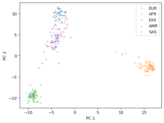
In the example below, we will use the PCA algorithm to reduce the dimensionality of a genetic dataset from the 1000 genomes project [1,2].
[1] Auton, A. et al. A global reference for human genetic variation. Nature 526, 68–74 (2015)
[2] Altshuler, D. M. et al. Integrating common and rare genetic variation in diverse human populations. Nature 467, 52–58 (2010)
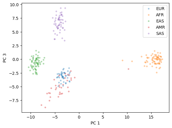
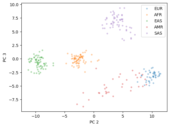
After reducing the dimensionality, we will plot the results and examine whether clusters of ancestries are visible.
We consider five ancestries in the dataset:
EUR - European
AFR - African
EAS - East Asian
SAS - South Asian
AMR - Native American
Show code cell source
snpreader = Bed('../../datasets/genetic_data_1kg/example2.bed', count_A1=True)
data = snpreader.read()
print(data.shape)
# y includes our labels and x includes our features
labels = pd.read_csv("../../datasets/genetic_data_1kg/1kg_annotations_edit.txt", sep="\t", index_col="Sample")
list1 = data.iid[:,1].tolist() #list with the Sample numbers present in genetic dataset
labels = labels[labels.index.isin(list1)] #filter labels DataFrame so it only contains the sampleIDs present in genetic data
y = labels.SuperPopulation # EUR, AFR, AMR, EAS, SAS
X = data.val[:, ~np.isnan(data.val).any(axis=0)] #load genetic data to X, removing NaN values
pca = PCA()
pca.fit(X=X)
X_pc = pca.transform(X)
X_reconstruction_full = pca.reverse_transform(X_pc)
print("L1 reconstruction error for full PCA : %.4E " % (np.absolute(X - X_reconstruction_full).sum()))
for rank in range(5): #more correct: X_pc.shape[1]+1
pca_lowrank = PCA(k=rank)
pca_lowrank.fit(X=X)
X_lowrank = pca_lowrank.transform(X)
X_reconstruction = pca_lowrank.reverse_transform(X_lowrank)
print("L1 reconstruction error for rank %i PCA : %.4E " % (rank, np.absolute(X - X_reconstruction).sum()))
fig = plt.figure()
plt.plot(X_pc[y=="EUR"][:,0], X_pc[y=="EUR"][:,1],'.', alpha = 0.3)
plt.plot(X_pc[y=="AFR"][:,0], X_pc[y=="AFR"][:,1],'.', alpha = 0.3)
plt.plot(X_pc[y=="EAS"][:,0], X_pc[y=="EAS"][:,1],'.', alpha = 0.3)
plt.plot(X_pc[y=="AMR"][:,0], X_pc[y=="AMR"][:,1],'.', alpha = 0.3)
plt.plot(X_pc[y=="SAS"][:,0], X_pc[y=="SAS"][:,1],'.', alpha = 0.3)
plt.xlabel("PC 1")
plt.ylabel("PC 2")
plt.legend(["EUR", "AFR","EAS","AMR","SAS"])
fig2 = plt.figure()
plt.plot(X_pc[y=="EUR"][:,0], X_pc[y=="EUR"][:,2],'.', alpha = 0.3)
plt.plot(X_pc[y=="AFR"][:,0], X_pc[y=="AFR"][:,2],'.', alpha = 0.3)
plt.plot(X_pc[y=="EAS"][:,0], X_pc[y=="EAS"][:,2],'.', alpha = 0.3)
plt.plot(X_pc[y=="AMR"][:,0], X_pc[y=="AMR"][:,2],'.', alpha = 0.3)
plt.plot(X_pc[y=="SAS"][:,0], X_pc[y=="SAS"][:,2],'.', alpha = 0.3)
plt.xlabel("PC 1")
plt.ylabel("PC 3")
plt.legend(["EUR", "AFR","EAS","AMR","SAS"])
fig3 = plt.figure()
plt.plot(X_pc[y=="EUR"][:,1], X_pc[y=="EUR"][:,2],'.', alpha = 0.3)
plt.plot(X_pc[y=="AFR"][:,1], X_pc[y=="AFR"][:,2],'.', alpha = 0.3)
plt.plot(X_pc[y=="EAS"][:,1], X_pc[y=="EAS"][:,2],'.', alpha = 0.3)
plt.plot(X_pc[y=="AMR"][:,1], X_pc[y=="AMR"][:,2],'.', alpha = 0.3)
plt.plot(X_pc[y=="SAS"][:,1], X_pc[y=="SAS"][:,2],'.', alpha = 0.3)
plt.xlabel("PC 2")
plt.ylabel("PC 3")
plt.legend(["EUR", "AFR","EAS","AMR","SAS"])
fig4 = plt.figure()
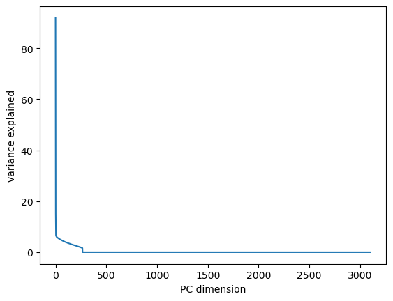
plt.plot(pca.variance_explained())
plt.xlabel("PC dimension")
plt.ylabel("variance explained")
fig4 = plt.figure()
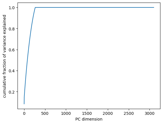
plt.plot(pca.variance_explained().cumsum() / pca.variance_explained().sum())
plt.xlabel("PC dimension")
plt.ylabel("cumulative fraction of variance explained")
plt.show()
(267, 10626)
L1 reconstruction error for full PCA : 1.3924E-09
L1 reconstruction error for rank 0 PCA : 3.7316E+05
L1 reconstruction error for rank 1 PCA : 3.4989E+05
L1 reconstruction error for rank 2 PCA : 3.3704E+05
L1 reconstruction error for rank 3 PCA : 3.3322E+05
L1 reconstruction error for rank 4 PCA : 3.3049E+05