Random variables#
A random variable is some uncertain quantity with an associated probability distribution over the values it can assume.
Formally, a random variable on a probability space \((\Omega, \mathcal{F}, \mathbb{P})\) is a function \(X: \Omega \to \mathbb{R}\).
We denote the range of \(X\) by \(X(\Omega) = \{X(\omega) : \omega \in \Omega\}\).
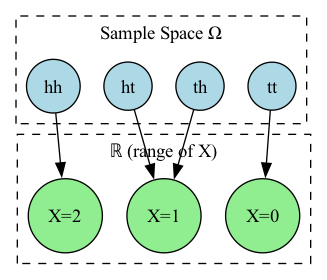
To give a concrete example, suppose \(X\) is the number of heads in two tosses of a fair coin.
The sample space is
and \(X\) is determined completely by the outcome \(\omega\), i.e. \(X = X(\omega)\).
For example, the event \(X = 1\) is the set of outcomes \(\{ht, th\}\).
Below is a visualization of the random variable \(X\) mapping the sample space \(\Omega\) to the real numbers \(\mathbb{R}\).
Show code cell source
from graphviz import Digraph

def plot_random_variable_graphviz():
    dot = Digraph(comment='Random Variable Mapping X: Ω → ℝ')

    omega = ['hh', 'ht', 'th', 'tt']
    X_map = {
        'hh': '2',
        'ht': '1',
        'th': '1',
        'tt': '0'
    }

    with dot.subgraph(name='cluster_omega') as c1:
        c1.attr(label='Sample Space Ω', style='dashed')
        for o in omega:
            c1.node(o, shape='circle', style='filled', fillcolor='lightblue')

    with dot.subgraph(name='cluster_real') as c2:
        c2.attr(label='ℝ (range of X)', style='dashed')
        for x in sorted(set(X_map.values())):
            c2.node(f'X={x}', shape='circle', style='filled', fillcolor='lightgreen')

    for w, x in X_map.items():
        dot.edge(w, f'X={x}')

    return dot

dot = plot_random_variable_graphviz()
# dot.render('random_variable_mapping', view=True, format='png')  # Creates PNG and opens it

from IPython.display import Image
dot.format = 'png'
dot.render('random_variable_mapping')
Image(filename='random_variable_mapping.png')
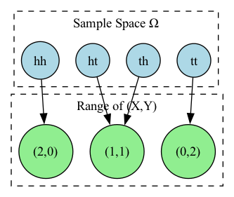
It is possible to define multiple random variables on the same probability space.
For example, we can define the random variable \(Y\) to be the number of tails in two tosses of a fair coin.
The sample space is still
and \(Y\) is determined completely by the outcome \(\omega\), i.e. \(Y = Y(\omega)\).
Below is a visualization of the joint random variable \((X, Y)\) mapping the sample space \(\Omega\) to the real numbers \(\mathbb{R}^2\).
Show code cell source
from graphviz import Digraph

def plot_joint_variable_graphviz():
    dot = Digraph(comment='Joint Random Variable Mapping: ω ↦ (X(ω), Y(ω))')

    omega = ['hh', 'ht', 'th', 'tt']
    joint_values = {
        'hh': (2, 0),
        'ht': (1, 1),
        'th': (1, 1),
        'tt': (0, 2)
    }

    # Subgraph for Ω
    with dot.subgraph(name='cluster_omega') as c1:
        c1.attr(label='Sample Space Ω', style='dashed')
        for o in omega:
            c1.node(o, shape='circle', style='filled', fillcolor='lightblue')

    # Subgraph for ℝ² (range of (X,Y))
    with dot.subgraph(name='cluster_range') as c2:
        c2.attr(label='Range of (X,Y)', style='dashed')
        unique_pairs = sorted(set(joint_values.values()))
        for (x, y) in unique_pairs:
            label = f'({x},{y})'
            c2.node(label, shape='circle', style='filled', fillcolor='lightgreen')

    # Edges: ω → (X(ω), Y(ω))
    for o in omega:
        x, y = joint_values[o]
        dot.edge(o, f'({x},{y})')

    return dot

dot = plot_joint_variable_graphviz()
# dot.render('joint_random_variable_mapping', view=True, format='png')  # Creates PNG and opens it

from IPython.display import Image
dot.format = 'png'
dot.render('joint_random_variable_mapping')
Image(filename='joint_random_variable_mapping.png')
It is common to talk about the values of a random variable without directly referencing its sample space. The two are related by the following definition: the event that the value of \(X\) lies in some set \(S \subseteq \mathbb{R}\) is
Note that special cases of this definition include \(X\) being equal to, less than, or greater than some specified value.
For example,
A word on notation: we write \(p(X)\) to denote the entire probability distribution of \(X\) and \(p(x)\) for the evaluation of the function \(p\) at a particular value \(x \in X(\Omega)\).
If \(p\) is parameterized by some parameters \(\theta\), we write \(p(X; \mathbf{\theta})\) or \(p(x; \mathbf{\theta})\), unless we are in a Bayesian setting where the parameters are considered a random variable, in which case we condition on the parameters.
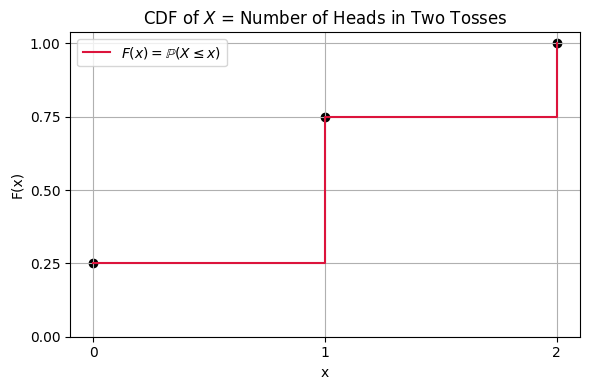
The cumulative distribution function#
The cumulative distribution function (c.d.f.) gives the probability that a random variable is at most a certain value:
The c.d.f. is a non-decreasing function that is right-continuous.
Show code cell source
import numpy as np
import matplotlib.pyplot as plt

# Discrete outcomes of X = number of heads in two tosses
x_vals = np.array([0, 1, 2])
pmf_vals = np.array([0.25, 0.5, 0.25])  # From outcomes: tt, ht/th, hh
cdf_vals = np.cumsum(pmf_vals)

# CDF step plot
plt.figure(figsize=(6, 4))
plt.step(x_vals, cdf_vals, where='post', label=r'$F(x) = \mathbb{P}(X \leq x)$', color='crimson')
plt.scatter(x_vals, cdf_vals, color='black')
plt.xticks([0, 1, 2])
plt.yticks(np.linspace(0, 1, 5))
plt.xlabel('x')
plt.ylabel('F(x)')
plt.title('CDF of $X$ = Number of Heads in Two Tosses')
plt.grid(True)
plt.legend()
plt.tight_layout()
plt.show()
The c.d.f. can be used to give the probability that a variable lies within a certain range:
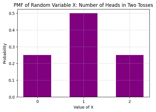
Discrete random variables#
A discrete random variable is a random variable that has a countable range and assumes each value in this range with positive probability.
Discrete random variables are completely specified by their probability mass function (p.m.f.) \(p : X(\Omega) \to [0,1]\) which satisfies
For a discrete \(X\), the probability of a particular value is given exactly by its p.m.f.:
Going back to our example. Below, we visualize the probability mass function (PMF) of \(X\), which gives the probability of each value of \(X\).
Show code cell source
import matplotlib.pyplot as plt

def plot_pmf():
    from collections import Counter

    omega = ['hh', 'ht', 'th', 'tt']
    X_values = [2 if o == 'hh' else 1 if o in ['ht', 'th'] else 0 for o in omega]
    probs = Counter(X_values)

    # Normalize
    for k in probs:
        probs[k] /= len(omega)

    plt.figure(figsize=(6, 4))
    plt.bar(probs.keys(), probs.values(), color='purple', width=0.6)
    plt.xlabel('Value of X')
    plt.ylabel('Probability')
    plt.xticks([0, 1, 2])
    plt.title('PMF of Random Variable X: Number of Heads in Two Tosses')
    plt.grid(True, linestyle='--', alpha=0.6)
    plt.show()
plot_pmf()
Continuous random variables#
A continuous random variable is a random variable that has an uncountable range and assumes each value in this range with probability zero.
Most of the continuous random variables that one would encounter in practice are absolutely continuous random variables, which means that there exists a function \(p : \mathbb{R} \to [0,\infty)\) that satisfies
The function \(p\) is called a probability density function (abbreviated p.d.f.) and must satisfy
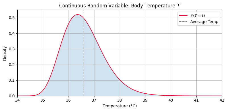
As an example for a continuous random variable, consider patient body temperature in a hospital.
Let
\(\Omega\): all possible physiological states of a patient at a point in time (heart rate, immune response, infection status, etc.)
\(\mathcal{F}\): a \(\sigma\)-algebra over measurable subsets of these states
\(\mathbb{P}\): probability measure capturing likelihoods over patient states
Define the random variable:
that maps each state \(\omega \in \Omega\) to a measured body temperature, e.g.,
Typical human temperatures range roughly between:
The average temperature in the United States is around 36.6°C, but there is some spread around this value and the distribution is not symmetric. Below is a visualization of the probability density function of the body temperature distribution (modelled as a gamma distribution).
Show code cell source
import numpy as np
import matplotlib.pyplot as plt
from scipy.stats import gamma
mean, sigma = 36.6, 0.8  # Mean and std dev of normal
min_temp = 34.0
max_temp = 42.0
loc = min_temp
var = sigma**2
theta = var / (mean - loc)
beta = 1.0 / theta
alpha = (mean - loc) / theta

def plot_body_temperature_pdf():


    # mean = alpha * theta + loc
    # var = alpha * theta**2

    # alpha * theta  = (mean - loc)
    # alpha = (mean - loc) / theta
    # alpha * theta**2 = var
    # (mean - loc) / theta * theta**2 = var
    # (mean - loc) * theta = var

    # print(alpha * theta + loc)
    # print(alpha * theta**2)

    x = np.linspace(min_temp, max_temp, 1000)
    y = gamma.pdf(x, loc = loc, scale=theta, a=alpha)

    plt.figure(figsize=(8, 4))
    plt.plot(x, y, label=r'$\mathbb{P}(T=t)$', color='crimson')
    plt.axvline(mean, color='gray', linestyle='--', label='Average Temp')
    plt.fill_between(x, y, alpha=0.2)
    plt.title('Continuous Random Variable: Body Temperature $T$')
    plt.xlabel('Temperature (°C)')
    plt.ylabel('Density')
    plt.legend()
    plt.grid(True)
    plt.tight_layout()
    plt.xlim(34, 42)
    plt.ylim(0, 0.55)
    plt.show()
def plot_body_temperature_cdf():
    x = np.linspace(min_temp, max_temp, 1000)
    y = gamma.cdf(x, loc = loc, scale=theta, a=alpha)
    plt.figure(figsize=(8, 4))
    plt.plot(x, y, label=r'$\mathbb{P}(T\leq t)$', color='crimson')
    plt.axvline(mean, color='gray', linestyle='--', label='Average Temp')
    plt.title('Cumulative Distribution Function of Body Temperature $T$')
    plt.xlabel('Temperature (°C)')
    plt.ylabel('Cumulative Probability')
    plt.legend()
    plt.grid(True)
    plt.tight_layout()
    plt.xlim(34, 42)
    plt.ylim(0, 1)
    plt.show()

plot_body_temperature_pdf()
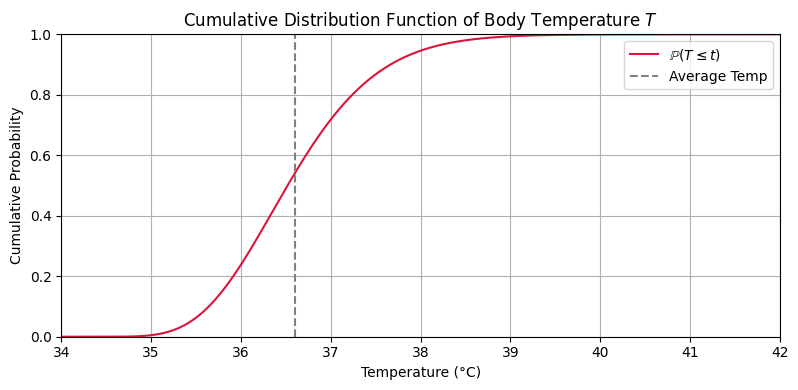
Below is a visualization of the cumulative distribution function of the body temperature distribution.
Show code cell source
plot_body_temperature_cdf()
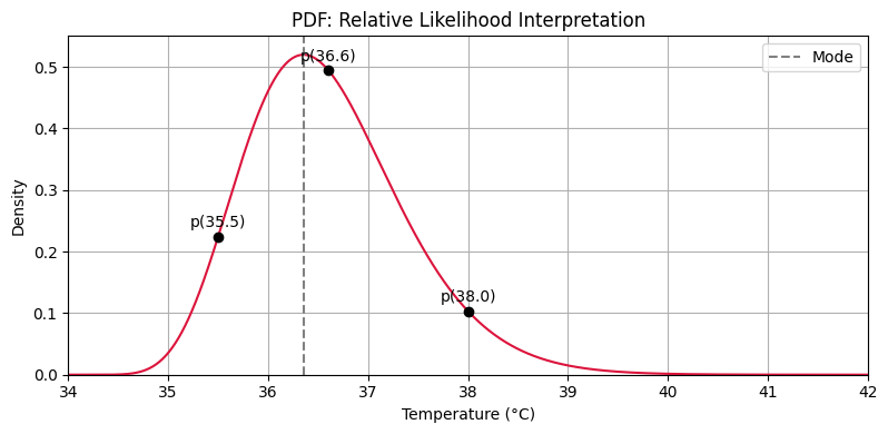
The values of the probability density function are not themselves probabilities, since they could exceed 1.
However, they do have a couple of reasonable interpretations.
One is as relative probabilities; even though the probability of each particular value being picked is technically zero, some points are still in a sense more likely than others.
Show code cell source
def plot_relative_likelihood():
    x = np.linspace(min_temp, max_temp, 1000)
    y = gamma.pdf(x, loc=loc, scale=theta, a=alpha)
    peak = x[np.argmax(y)]

    plt.figure(figsize=(8, 4))
    plt.plot(x, y, color='crimson')
    plt.title('PDF: Relative Likelihood Interpretation')
    plt.xlabel('Temperature (°C)')
    plt.ylabel('Density')
    plt.grid(True)

    # Highlight three points
    for temp in [35.5, 36.6, 38.0]:
        fx = gamma.pdf(temp, loc=loc, scale=theta, a=alpha)
        plt.plot([temp], [fx], marker='o', color='black')
        plt.text(temp, fx + 0.015, f'p({temp:.1f})', ha='center')

    plt.axvline(peak, color='gray', linestyle='--', label='Mode')
    plt.legend()
    plt.tight_layout()
    plt.xlim(34, 42)
    plt.ylim(0, 0.55)
    plt.show()

plot_relative_likelihood()
One can also think of the density as determining the probability that the variable will lie in a small range about a given value. This is because, for small \(\epsilon > 0\),
using a midpoint approximation to the integral.
Show code cell source
def plot_density_as_probability():
    x = np.linspace(min_temp, max_temp, 1000)
    y = gamma.pdf(x, loc=loc, scale=theta, a=alpha)

    center = 37.0
    epsilon = 0.2
    a, b = center - epsilon, center + epsilon

    # True probability via integration
    prob_true = gamma.cdf(b, loc=loc, scale=theta, a=alpha) - gamma.cdf(a, loc=loc, scale=theta, a=alpha)
    approx = 2 * epsilon * gamma.pdf(center, loc=loc, scale=theta, a=alpha)

    plt.figure(figsize=(8, 4))
    plt.plot(x, y, label='PDF', color='crimson')
    plt.fill_between(x, y, where=(x >= a) & (x <= b), color='orange', alpha=0.4, label='~P(x ∈ [x−ε, x+ε])')
    plt.axvline(center, color='gray', linestyle='--', label=f'x = {center}')
    plt.title(r'$\mathbb{{P}}(x-\epsilon \leq X \leq x+\epsilon) \approx 2\epsilon \cdot p(x)$')
    plt.xlabel('Temperature (°C)')
    plt.ylabel('Density')
    plt.legend()
    plt.grid(True)
    plt.tight_layout()
    plt.xlim(34, 42)
    plt.ylim(0, 0.55)
    plt.show()

    print(f"True probability ≈ {prob_true:.4f}, Midpoint approx ≈ {approx:.4f}")

plot_density_as_probability()
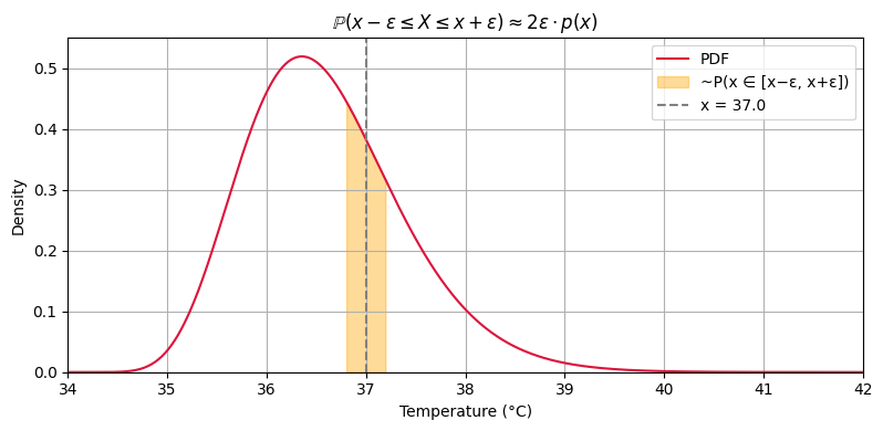
True probability ≈ 0.1528, Midpoint approx ≈ 0.1531
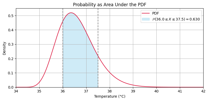
Here are some useful identities that follow from the definitions above:
Show code cell source
def plot_area_probability():
    x = np.linspace(min_temp, max_temp, 1000)
    y = gamma.pdf(x, loc=loc, scale=theta, a=alpha)

    a, b = 36.0, 37.5
    prob = gamma.cdf(b, loc=loc, scale=theta, a=alpha) - gamma.cdf(a, loc=loc, scale=theta, a=alpha)

    plt.figure(figsize=(8, 4))
    plt.plot(x, y, label='PDF', color='crimson')
    plt.fill_between(x, y, where=(x >= a) & (x <= b), color='skyblue', alpha=0.4,
                     label=fr'$\mathbb{{P}}({a} \leq X \leq {b}) \approx {prob:.3f}$')
    plt.axvline(a, color='gray', linestyle='--')
    plt.axvline(b, color='gray', linestyle='--')
    plt.title('Probability as Area Under the PDF')
    plt.xlabel('Temperature (°C)')
    plt.ylabel('Density')
    plt.legend()
    plt.grid(True)
    plt.tight_layout()
    plt.xlim(34, 42)
    plt.ylim(0, 0.55)
    plt.show()

plot_area_probability()
Other kinds of random variables#
There are random variables that are neither discrete nor continuous. For example, consider a random variable determined as follows: flip a fair coin, then the value is zero if it comes up heads, otherwise draw a number uniformly at random from \([1,2]\). Such a random variable can take on uncountably many values, but only finitely many of these with positive probability.
We will not discuss such random variables because they are rather pathological and require measure theory to analyze.