Determinant

The determinant is a scalar quantity associated with any square matrix \(\mathbf{A} \in \mathbb{R}^{n \times n}\). It encodes important geometric and algebraic information about the transformation represented by \(\mathbf{A}\).

Geometrically, the determinant tells us:

• How the matrix \(\mathbf{A}\) scales volume: The absolute value \(|\det(\mathbf{A})|\) is the volume-scaling factor for the linear transformation \(\mathbf{x} \mapsto \mathbf{A}\mathbf{x}\).

• Whether the transformation preserves or flips orientation: If \(\det(\mathbf{A}) > 0\), the transformation preserves orientation; if \(\det(\mathbf{A}) < 0\), it reverses it (like a reflection).

Algebraically, the determinant can be defined as:

\[ \det(\mathbf{A}) = \sum_{\sigma \in S_n} \operatorname{sgn}(\sigma) \cdot a_{1\sigma(1)} a_{2\sigma(2)} \cdots a_{n\sigma(n)} \]

where:

• The sum is over all permutations \(\sigma\) of \(\{1, 2, \dots, n\}\),

• \(\operatorname{sgn}(\sigma)\) is \(+1\) or \(-1\) depending on the parity of the permutation.

This formula is computationally expensive and confusing, but conceptually important: it captures how the determinant depends on all possible signed products of entries, each taken once from a distinct row and column.

Let’s illustrate the determinant geometrically.

Show code cell source Hide code cell source

import numpy as np
import matplotlib.pyplot as plt
from matplotlib.patches import Polygon

# Define matrices to show area effects
matrices = {
    "Area = 1 (Identity)": np.array([[1, 0], [0, 1]]),
    "Area > 1": np.array([[2, 0.5], [0.5, 1.5]]),
    "Area < 0 (Flip)": np.array([[0, 1], [1, 0]]),
    "Rotation (Area = 1)": np.array([[np.cos(np.pi/4), -np.sin(np.pi/4)],
                                     [np.sin(np.pi/4),  np.cos(np.pi/4)]])
}

# Unit square
square = np.array([[0, 0],
                   [1, 0],
                   [1, 1],
                   [0, 1],
                   [0, 0]]).T

fig, axes = plt.subplots(1, 4, figsize=(20, 5))

for ax, (title, M) in zip(axes, matrices.items()):
    transformed_square = M @ square
    area = np.abs(np.linalg.det(M))
    det = np.linalg.det(M)

    # Plot original unit square
    ax.plot(square[0], square[1], 'k--', label='Unit square')
    ax.fill(square[0], square[1], facecolor='lightgray', alpha=0.4)

    # Plot transformed shape
    ax.plot(transformed_square[0], transformed_square[1], 'b-', label='Transformed')
    ax.fill(transformed_square[0], transformed_square[1], facecolor='skyblue', alpha=0.6)

    # Add vector arrows for columns of M
    origin = np.array([[0, 0]]).T
    for i in range(2):
        vec = M[:, i]
        ax.quiver(*origin, vec[0], vec[1], angles='xy', scale_units='xy', scale=1, color='red')

    ax.set_title(f"{title}\nDet = {det:.2f}, Area = {area:.2f}")
    ax.set_xlim(-2, 3)
    ax.set_ylim(-2, 3)
    ax.set_aspect('equal')
    ax.grid(True)
    ax.legend()

plt.suptitle("Geometric Interpretation of the Determinant (Area Scaling and Orientation)", fontsize=16)
plt.tight_layout(rect=[0, 0, 1, 0.93])
plt.show()

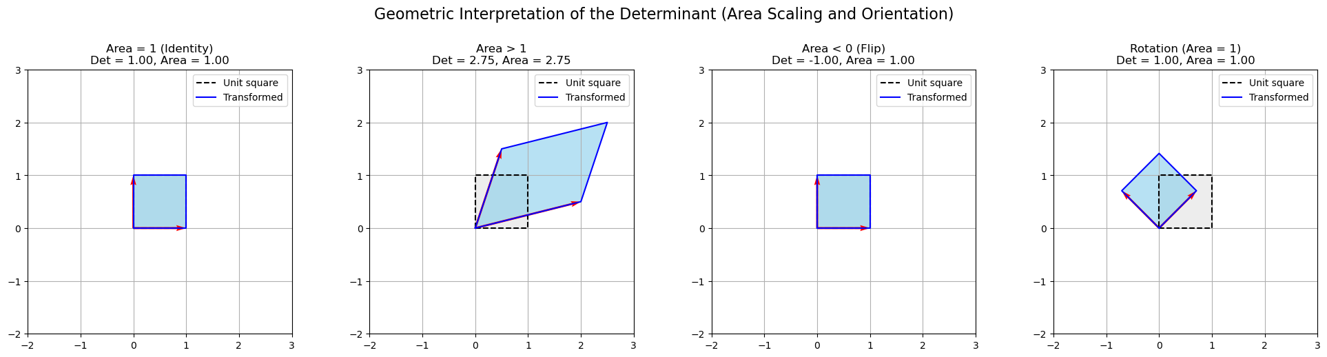
1. Identity: No change — area = 1.

2. Stretch: Expands area — determinant > 1.

3. Flip: Reflects across the diagonal — determinant < 0.

4. Rotation: Rotates without distortion — determinant = 1.

What is the Determinant?

The determinant of a matrix \(\mathbf{A} \in \mathbb{R}^{n \times n}\) is a scalar that describes how \(\mathbf{A}\) scales space. Algebraically, it is defined by a signed sum over all permutations of the matrix’s entries. Geometrically, it quantifies the change in signed volume of a unit shape under transformation by \(\mathbf{A}\). If the determinant is zero, the transformation collapses the volume entirely, and \(\mathbf{A}\) is singular (non-invertible).

---

The determinant has several important properties:

(i) \(\det(\mathbf{I}) = 1\)

(ii) \(\det(\mathbf{A}^{\!\top\!}) = \det(\mathbf{A})\)

(iii) \(\det(\mathbf{A}\mathbf{B}) = \det(\mathbf{A})\det(\mathbf{B})\)

(iv) \(\det(\mathbf{A}^{-1}) = \det(\mathbf{A})^{-1}\)

(v) \(\det(\alpha\mathbf{A}) = \alpha^n \det(\mathbf{A})\)

---

Practical Computation of the Determinant

The algebraic definition of the determinant is computationally expensive. In practice, we compute the determinant using property (iii) and a matrix factorization such as the PLU decomposition:

\[ \mathbf{A} = \mathbf{P} \mathbf{L} \mathbf{U} \]

where \(\mathbf{P}\) is a permutation matrix, \(\mathbf{L}\) is a unit lower triangular matrix, and \(\mathbf{U}\) is an upper triangular matrix.

Theorem (Triangular Matrix Determinant)

Let \(\mathbf{T} \in \mathbb{R}^{n \times n}\) be a triangular matrix, either upper or lower triangular.

Then:

\[ \boxed{ \det(\mathbf{T}) = \prod_{i=1}^n T_{ii} } \]

Then,

\[ \boxed{ \det(\mathbf{A}) = \det(\mathbf{P}) \cdot \det(\mathbf{L}) \cdot \det(\mathbf{U}) } \]

Since:

• \(\det(\mathbf{L}) = 1\) (if unit lower triangular),

• \(\det(\mathbf{U}) = \prod_{i=1}^n u_{ii}\),

• \(\det(\mathbf{P}) = (-1)^s\), where \(s\) is the number of row swaps,

this method reduces determinant computation to \(\mathcal{O}(n)\) operations after LU decomposition. As the cost for the LU decomposition is \(\mathcal{O}(n^3),\) the total cost of computing the determinant is \(\mathcal{O}(n^3).\)

Cofactor Expansion: Definition

Cofactor expansion (also called Laplace expansion) gives a recursive definition of the determinant.

Let \(\mathbf{A} \in \mathbb{R}^{n \times n}\) be a square matrix.

Then the determinant of \(\mathbf{A}\) can be computed by expanding along any row or column.

For simplicity, we’ll define it for the first column.

\[ \boxed{ \det(\mathbf{A}) = \sum_{i=1}^{n} (-1)^{i+1} \cdot A_{i1} \cdot \det(\mathbf{A}^{(i,1)}) } \]

Where:

• \(A_{i1}\) is the entry in row \(i\), column 1

• \(\mathbf{A}^{(i,1)}\) is the minor matrix obtained by deleting row \(i\) and column 1 from \(\mathbf{A}\)

• \((-1)^{i+1}\) is the sign factor for alternating signs (from the checkerboard sign pattern)

• \((-1)^{i+j} \cdot \det(\mathbf{A}^{(i,j)})\) is called the cofactor of \(A_{ij}\)

This formula recursively reduces the computation of a determinant to smaller and smaller submatrices.

---

Cofactor Expantion Example (3×3 Matrix)

Let:

\[\begin{split} \mathbf{A} = \begin{bmatrix} 1 & 2 & 3 \\ 4 & 5 & 6 \\ 7 & 8 & 9 \end{bmatrix} \end{split}\]

Expand along the first column:

\[\begin{split} \det(\mathbf{A}) = (+1) \cdot 1 \cdot \begin{vmatrix} 5 & 6 \\ 8 & 9 \end{vmatrix} - 4 \cdot \begin{vmatrix} 2 & 3 \\ 8 & 9 \end{vmatrix} + 7 \cdot \begin{vmatrix} 2 & 3 \\ 5 & 6 \end{vmatrix} \end{split}\]

Now compute the 2×2 determinants:

\[ \det(\mathbf{A}) = 1 \cdot (5 \cdot 9 - 6 \cdot 8) - 4 \cdot (2 \cdot 9 - 3 \cdot 8) + 7 \cdot (2 \cdot 6 - 3 \cdot 5) \]

\[ = 1 \cdot (-3) - 4 \cdot (-6) + 7 \cdot (-3) = -3 + 24 - 21 = 0 \]

So:

\[ \boxed{\det(\mathbf{A}) = 0} \]

Proof. via Laplace Expansion / Cofactor Expansion

We’ll prove this for upper triangular matrices by induction on the matrix size \(n\). The same argument applies symmetrically for lower triangular matrices.

---

Base Case: \(n = 1\)

Let \(\mathbf{T} = [t_{11}]\). Then clearly:

\[ \det(\mathbf{T}) = t_{11} = \prod_{i=1}^1 T_{ii} \]

The base case holds.

---

Inductive Step

Assume the result holds for \((n-1) \times (n-1)\) upper triangular matrices.

Now let \(\mathbf{T} \in \mathbb{R}^{n \times n}\) be upper triangular. That means all entries below the diagonal are zero:

\[\begin{split} \mathbf{T} = \begin{bmatrix} t_{11} & t_{12} & \dots & t_{1n} \\ 0 & t_{22} & \dots & t_{2n} \\ \vdots & \vdots & \ddots & \vdots \\ 0 & 0 & \dots & t_{nn} \end{bmatrix} \end{split}\]

Use cofactor expansion along the first column. Since the only nonzero entry in the first column is \(t_{11}\), we have:

\[ \det(\mathbf{T}) = t_{11} \cdot \det(\mathbf{T}^{(1,1)}) \]

Where \(\mathbf{T}^{(1,1)}\) is the \((n-1)\times(n-1)\) matrix obtained by deleting row 1 and column 1. But:

• \(\mathbf{T}^{(1,1)}\) is still upper triangular.

• By the inductive hypothesis:

  \[ \det(\mathbf{T}^{(1,1)}) = \prod_{i=2}^{n} T_{ii} \]

So:

\[ \det(\mathbf{T}) = t_{11} \cdot \prod_{i=2}^{n} T_{ii} = \prod_{i=1}^{n} T_{ii} \]

The inductive step holds.

---

Conclusion

By induction, for any upper (or lower) triangular matrix \(\mathbf{T} \in \mathbb{R}^{n \times n}\),

\[ \boxed{ \det(\mathbf{T}) = \prod_{i=1}^n T_{ii} } \]

• The determinant accumulates only the diagonal entries because each pivot is isolated, and all other paths in the expansion have zero entries.

• This result is frequently used in:

  • Computing determinants from LU decomposition

  • Checking invertibility efficiently

  • Proving properties of eigenvalues and characteristic polynomials