Building a BFGS Optimizer from Scratch#
🌟 Motivation#
Optimization lies at the heart of machine learning. Every model we train—whether it’s a linear regression, logistic regression, or a deep neural network—relies fundamentally on efficient algorithms to minimize error and find the best parameters.
You’ve learned about gradient descent, which is intuitive but can be slow and sensitive to step sizes.
You’ve also briefly touched on Newton’s method, powerful but computationally expensive due to the need for second derivatives (Hessians).
Can we get the rapid convergence benefits of Newton’s method without explicitly computing expensive Hessians? Yes—this is exactly the motivation behind Quasi-Newton methods, and in particular, the widely-used BFGS algorithm.
BFGS intelligently approximates curvature information, providing fast and stable convergence without explicitly computing second derivatives.
It’s widely used in practice due to its reliability, speed, and simplicity of implementation.
By implementing your own BFGS optimizer from scratch, you’ll gain deep, practical insights into how powerful optimization methods really work, enhancing both your mathematical intuition and programming skills.
Show code cell source
import numpy as np
import matplotlib.pyplot as plt
from scipy.optimize import minimize

# Define the Rosenbrock function
def rosenbrock(x):
    return (1 - x[0])**2 + 100 * (x[1] - x[0]**2)**2

# Store optimization path
trajectory = []

def callback(xk):
    trajectory.append(np.copy(xk))

# Initial guess
x0 = np.array([-1.5, 1.5])
trajectory.append(np.copy(x0))

# Run BFGS
res = minimize(rosenbrock, x0, method='BFGS', callback=callback, options={'disp': False})

# Convert trajectory to array
trajectory = np.array(trajectory)

# Create contour plot
x = np.linspace(-2, 2, 400)
y = np.linspace(-1, 3, 400)
X, Y = np.meshgrid(x, y)
Z = (1 - X)**2 + 100 * (Y - X**2)**2

ax = plt.figure(figsize=(8, 6))
plt.contour(X, Y, Z, levels=np.logspace(-0.5, 3.5, 30), cmap='viridis')
plt.plot(trajectory[:, 0], trajectory[:, 1], 'r.-', label='BFGS Path')
plt.quiver(trajectory[:-1, 0], trajectory[:-1, 1],
           trajectory[1:, 0] - trajectory[:-1, 0],
           trajectory[1:, 1] - trajectory[:-1, 1],
           scale_units='xy', angles='xy', scale=1, color='red')
plt.plot([1], [1], 'bo', label='Minimum')
plt.xlabel('$x_1$')
plt.ylabel('$x_2$')

plt.title('BFGS Optimization Path on Rosenbrock Function')
plt.legend()
plt.grid(True)
# plt.axis('equal')
plt.tight_layout()
plt.xlim(-2,2)
plt.show()
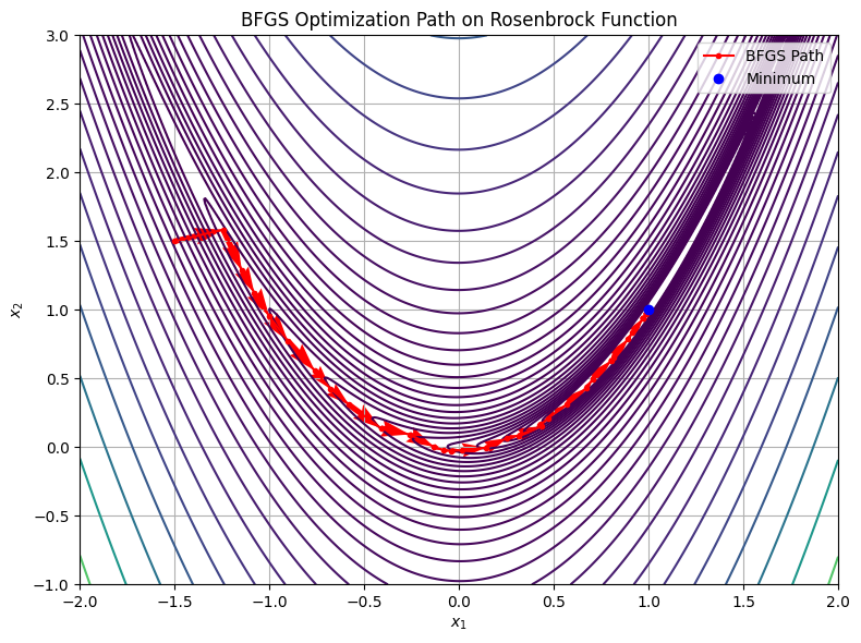
Here’s a visual summary of the BFGS optimization trajectory on the Rosenbrock function:
The contours show the curved shape of the loss surface.
The red arrows trace the optimization path.
The blue dot marks the global minimum at \((1, 1)\).
This nicely illustrates:
Curvature-aware updates of BFGS,
Faster convergence compared to plain gradient descent,
The impact of Hessian approximations in navigating challenging geometry.
📌 What You Will Do in This Project#
Your clear and concrete goal is:
Implement the BFGS optimization algorithm from scratch using NumPy, and evaluate it on classic optimization problems, including the Rosenbrock function and a small neural-network regression loss.
Specifically, you’ll:
Implement the full BFGS algorithm, clearly maintaining and updating a dense Hessian approximation matrix.
Integrate a robust line-search procedure that meets Wolfe conditions to ensure stable convergence.
Compare your custom NumPy implementation to the optimized SciPy implementation, assessing performance in terms of speed, stability, and convergence.
🔍 Key Concepts You’ll Master#
This project will give you practical mastery of several crucial optimization concepts:
Quasi-Newton approximation: Clearly understand how the BFGS method approximates Hessian matrices using just gradient evaluations, without computing expensive second derivatives.
BFGS update rule: Derive and implement the Hessian approximation update explicitly, clearly managing numerical stability.
Wolfe-condition line search: Learn how choosing appropriate step sizes ensures efficient and stable convergence in practice.
🚧 Core Tasks (Implementation Details)#
You’ll concretely engage with the following tasks:
BFGS Hessian approximation update: Implement the BFGS update rule from scratch, clearly managing the Hessian approximation matrix.
Line-search implementation: Integrate a robust Wolfe-condition line search to select stable step sizes along each direction.
Testing and benchmarking: Evaluate your optimizer on:
The Rosenbrock function, a classical optimization benchmark problem.
A small neural-network regression loss (e.g., 1-layer MLP).
Performance comparison: Compare clearly your BFGS implementation against SciPy’s BFGS implementation regarding speed, convergence, and numerical stability.
📝 Reporting: Analysis and Insights#
Your brief (~2 pages) report should include:
Clear explanations of how the BFGS curvature approximation works, and how this approximation compares to Gradient Descent (GD) and exact Hessian methods (Newton’s).
Performance comparison plots illustrating convergence rates and optimization behavior.
Discussion on your observations regarding stability, convergence speed, and potential issues (e.g., ill-conditioned Hessian approximations).
🚀 Stretch Goals (Optional, Advanced)#
For deeper insight and challenge, you could:
Implement the limited-memory BFGS (L-BFGS) method, clearly demonstrating reduced memory overhead and comparing performance to your full BFGS implementation.
Extend your implementation to handle bound-constraints (L-BFGS-B style) for optimization in a bounded domain.
📚 Resources and Support#
Starter code for Rosenbrock and simple neural network loss will be provided, allowing you to focus primarily on BFGS implementation and comparisons.
Feel free to utilize external resources, class notes, and clearly documented AI-assisted tools.
✅ Why This Matters#
Building your own BFGS optimizer deepens your understanding of numerical optimization:
It reinforces foundational mathematical concepts—gradient-based optimization, curvature approximation, and numerical stability.
It equips you with practical, hands-on experience that’s directly applicable in both academic research and industrial machine learning.
A self-implemented BFGS optimizer makes an impressive portfolio piece, demonstrating your capability in translating sophisticated theory into practical code.
Let’s dive in and build your very own BFGS optimizer!
Project Summary: Building a BFGS Optimizer#
(NumPy)
Item |
Details |
|---|---|
Goal |
Implement the full BFGS algorithm from scratch and test it on the Rosenbrock function and a small neural network regression loss. |
Key ideas |
Curvature approximation via Hessian updates, Wolfe-condition line search, comparison to GD and Newton methods. |
Core tasks |
|
Report |
Explain BFGS curvature updates and contrast with GD and Newton; include convergence plots and observations. |
Stretch |
Implement L-BFGS as a memory-efficient variant; optionally extend to L-BFGS-B for box constraints. |