Kernelized PCA#
🌟 Motivation#
Imagine you have data shaped like a spiral or a “Swiss-roll”—clearly non-linear, twisted, and curved. Ordinary PCA, as you’ve learned, excels at linear dimensionality reduction but will struggle with such nonlinear structures. What if we could extend PCA to discover the intrinsic, low-dimensional structure hidden within complex, nonlinear datasets?
Kernelized PCA is exactly the method we need:
It cleverly uses kernel methods to implicitly map data into high-dimensional feature spaces, where nonlinear relationships become linear.
Allows us to leverage PCA in that transformed space, giving us powerful nonlinear dimensionality reduction.
Uncovers hidden structure and simplifies the representation of data, which can be critical for downstream tasks like classification, visualization, or clustering.
Show code cell source
import numpy as np
import matplotlib.pyplot as plt
from sklearn.datasets import make_swiss_roll
from sklearn.decomposition import PCA, KernelPCA

# Generate Swiss roll data
X, color = make_swiss_roll(n_samples=1000, noise=0.05)
X = X[:, [0, 2]]  # Use only two dimensions (flattened roll)

# Apply linear PCA
pca = PCA(n_components=2)
X_pca = pca.fit_transform(X)

# Apply Kernel PCA with RBF kernel
kpca = KernelPCA(n_components=2, kernel="rbf", gamma=10)
X_kpca = kpca.fit_transform(X)

# Plotting
fig, axes = plt.subplots(1, 3, figsize=(15, 4.5))

axes[0].scatter(X[:, 0], X[:, 1], c=color, cmap=plt.cm.Spectral)
axes[0].set_title("Original Swiss Roll (2D slice)")
axes[0].set_xlabel("x")
axes[0].set_ylabel("z")

axes[1].scatter(X_pca[:, 0], X_pca[:, 1], c=color, cmap=plt.cm.Spectral)
axes[1].set_title("Linear PCA")
axes[1].set_xlabel("PC1")
axes[1].set_ylabel("PC2")

axes[2].scatter(X_kpca[:, 0], X_kpca[:, 1], c=color, cmap=plt.cm.Spectral)
axes[2].set_title("Kernel PCA (RBF)")
axes[2].set_xlabel("KPC1")
axes[2].set_ylabel("KPC2")

plt.tight_layout()
plt.show()
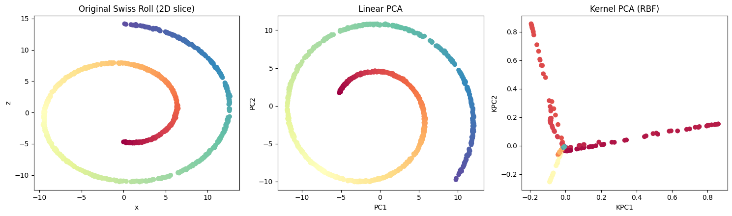
Here is a figure comparing:
A 2D slice of the original Swiss-roll structure.
The result of applying linear PCA (which fails to untangle the manifold).
The result of Kernel PCA with an RBF kernel, which successfully “unrolls” the manifold into a meaningful 2D representation.
This visual clearly highlights the power of nonlinear methods like KPCA over traditional PCA when dealing with complex, curved data.
📌 What You Will Do in This Project#
Your main goal is clear and concrete:
Implement Kernelized PCA using an RBF kernel and apply it to the classic nonlinear “Swiss-roll” dataset.
Specifically, you will:
Construct and center the kernel matrix using an RBF kernel.
Perform eigen-decomposition on the centered kernel matrix.
Project the data onto the top-2 eigenvectors to visualize the intrinsic low-dimensional structure clearly.
(Optionally) reconstruct original-space approximations (“pre-images”) using kernel regression.
🔍 Key Concepts You’ll Master#
You’ll gain practical experience with these fundamental concepts:
Kernel trick and nonlinear mapping: How to implicitly represent nonlinear data in high-dimensional feature spaces without explicitly computing the mapping.
Centering the kernel matrix: Why and how we need to center kernels in the implicit feature space.
Eigen-decomposition of kernels: The theoretical connection between the eigenvectors of the kernel matrix and nonlinear principal components.
RBF kernel and hyperparameters: Understanding the role of kernel width (γ) in capturing data complexity and nonlinear structure.
🚧 Core Tasks (Implementation Details)#
In practice, your workflow includes:
Constructing the Kernel Matrix: Implement the RBF (Gaussian) kernel function, then compute and center the kernel matrix \(K_c\).
Eigen-decomposition: Extract eigenvectors and eigenvalues from the centered kernel matrix. Identify and use the top-2 eigenvectors to project your data into 2-D.
Visualization and Interpretation: Produce clear scatter plots that demonstrate how KPCA captures the underlying nonlinear structure compared to linear PCA.
Optional but insightful:
Pre-image reconstruction: Implement a simple kernel regression approach to approximate how the 2-D latent coordinates relate back to original data space.
📝 Reporting: Analysis and Insights#
Your short report (~2 pages) should highlight clearly:
Derivation of the KPCA: Derive the KPCA from PCA using the kernel trick.
Linear PCA vs KPCA: Compare scatter plots to illustrate how KPCA recovers meaningful nonlinear structure missed by standard PCA.
Role of Kernel Parameter (γ): Discuss how varying γ influences the quality of dimensionality reduction and visualize this clearly.
Explained Variance: Include a brief analysis of explained variance from eigenvalues, demonstrating how effectively KPCA compresses information.
🚀 Stretch Goals (Optional, Advanced)#
To delve deeper, consider:
Conducting a systematic grid-search over γ and reporting how this affects the embedding quality and variance explained.
Exploring alternate kernels (polynomial, sigmoid) and comparing their performance on nonlinear datasets.
Explore probabilistic KPCA.
📚 Resources and Support#
You have access to provided datasets and basic visualization code to jumpstart your experimentation.
You’re encouraged to make use of external resources, lecture notes, and AI-assisted learning—clearly documented in your submission.
✅ Why This Matters#
By mastering Kernelized PCA, you’ll have:
Practical insight into kernel methods—crucial tools across machine learning.
An intuitive understanding of nonlinear dimensionality reduction, directly applicable to problems in visualization, clustering, or preprocessing.
An impressive and insightful component for your portfolio that demonstrates your ability to translate theory into clear, actionable implementation.
Project Summary: Kernelized PCA#
(NumPy)
Item |
Details |
|---|---|
Goal |
Implement KPCA with RBF kernel and project “Swiss-roll” data to 2-D. |
Key ideas |
Centering in feature space, eigen-decomposition of kernel matrix. |
Core tasks |
|
Report |
Contrast linear PCA vs. KPCA scatter plots; discuss role of \(\gamma\). |
Stretch |
Grid-search \(\gamma\) and report explained variance; explore probabilistic KPCA. |