Gaussian Mixture Models with EM#
🌟 Motivation#
Imagine you’re given data that clearly doesn’t come from a single Gaussian distribution. Instead, it forms multiple clusters, each with distinct shapes, sizes, and orientations. Gaussian Mixture Models (GMMs) provide a flexible, probabilistic approach for modeling exactly this type of complex data.
GMMs are widely used across machine learning tasks, including:
Clustering: Grouping data points into meaningful sub-populations.
Density estimation: Understanding underlying data structure in a probabilistic manner.
Anomaly detection: Identifying unusual data points based on probabilities.
To fit a GMM, you’ll use a powerful iterative procedure known as Expectation-Maximization (EM), which neatly handles missing information—here, the assignment of data points to Gaussian components.
Show code cell source
import numpy as np
import matplotlib.pyplot as plt
from sklearn.mixture import GaussianMixture
from sklearn.datasets import make_blobs
from matplotlib.patches import Ellipse

# Generate synthetic data
X, y_true = make_blobs(n_samples=500, centers=4, cluster_std=1.0, random_state=42)

# Fit GMM
gmm = GaussianMixture(n_components=4, covariance_type='full', random_state=42)
gmm.fit(X)
labels = gmm.predict(X)

# Plot data and Gaussian components
def plot_ellipse(mean, cov, ax, n_std=2.0, facecolor='none', **kwargs):
    vals, vecs = np.linalg.eigh(cov)
    order = vals.argsort()[::-1]
    vals, vecs = vals[order], vecs[:, order]
    angle = np.degrees(np.arctan2(*vecs[:,0][::-1]))
    width, height = 2 * n_std * np.sqrt(vals)
    ellipse = Ellipse(xy=mean, width=width, height=height, angle=angle, facecolor=facecolor, **kwargs)
    ax.add_patch(ellipse)

fig, ax = plt.subplots(figsize=(8, 6))
ax.scatter(X[:, 0], X[:, 1], c=labels, s=20, cmap='viridis', alpha=0.5)
for i in range(gmm.n_components):
    plot_ellipse(gmm.means_[i], gmm.covariances_[i], ax, edgecolor='black', linewidth=2)

ax.set_title('Gaussian Mixture Model with EM\n(Color = Component Assignment, Ellipses = 2σ Contours)')
ax.set_xlabel('X1')
ax.set_ylabel('X2')
plt.grid(True)
plt.tight_layout()
plt.show()
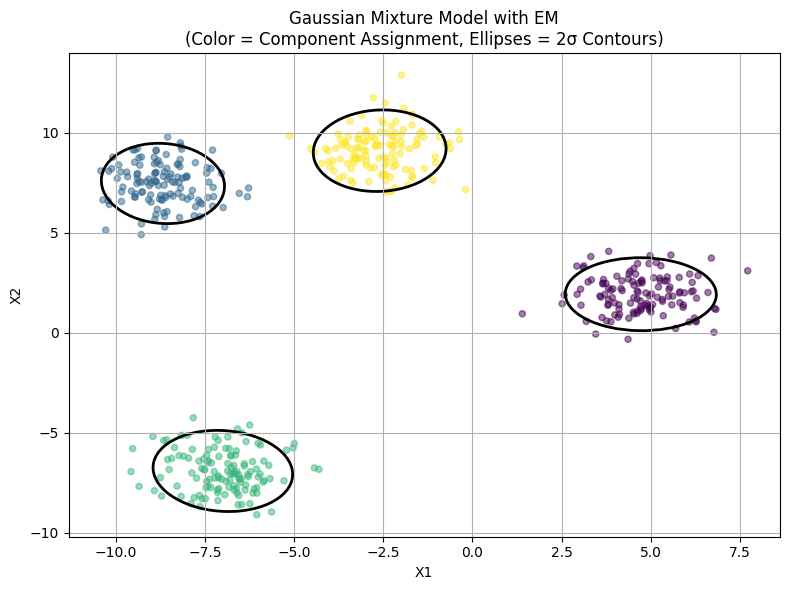
Here’s a figure visualizing the key concepts of Gaussian Mixture Models with the EM algorithm:
Colored points show the data assigned to each Gaussian component.
Black ellipses indicate the 2σ contours of each fitted Gaussian.
The model captures both the clustering and shape (covariance) of the components through iterative EM updates.
📌 What You Will Do in This Project#
Your core goal is clear:
Fit a 2-dimensional Gaussian Mixture Model using the EM algorithm, visualizing clearly how your model converges.
In this project you’ll implement from scratch (using NumPy only):
A Gaussian Mixture Model with 3 to 5 Gaussian components.
The full Expectation-Maximization algorithm, alternating between soft cluster assignments and Gaussian parameter updates.
A visualization tool to clearly show how your algorithm refines the clusters step-by-step.
🔍 Key Concepts You’ll Master#
This project introduces you to several foundational ideas in probabilistic machine learning:
Soft clustering (E-step): Unlike k-means (hard assignment), EM assigns data points to clusters probabilistically, capturing uncertainty explicitly.
Closed-form parameter updates (M-step): You’ll derive and implement exact, analytic updates for means, covariances, and cluster weights.
Numerical stability (log-sum-exp trick): Real-world implementations require care to avoid numerical underflow when computing probabilities. You’ll learn and apply the log-sum-exp trick.
🚧 Core Tasks (Implementation Details)#
You’ll follow these practical steps:
Expectation Step (E-step): Compute posterior probabilities (soft assignments) that each data point belongs to each cluster.
Maximization Step (M-step): Analytically update the means, covariances, and mixture weights from these probabilities.
Convergence and Visualization: Track the log-likelihood of the data under your model each iteration.
Plot the 2-sigma covariance ellipses of each Gaussian component every 5 iterations.
Observe how the components shift and reshape to fit the data.
Your implementation will show clearly how EM iteratively increases the likelihood and refines cluster boundaries.
📝 Reporting: Analysis and Insights#
Your short report (~2 pages) should clearly document:
Derivation of the GMM: Derive the GMM from first principles.
Derivation of the EM algorithm: Derive the EM algorithm from first principles.
Log-likelihood evolution: Plot the log-likelihood at each iteration to demonstrate monotonic convergence.
Discussion of convergence: Identify local optima and discuss strategies to mitigate this (e.g., initialization strategies or multiple runs).
Visualization interpretation: Explain how and why the Gaussian components change during EM.
🚀 Stretch Goals (Optional, Advanced)#
To further enrich your understanding, you might:
Implement Bayesian Information Criterion (BIC): Automatically determine the best number of clusters (K).
Explore initialization methods: Compare random initialization to k-means initialization and discuss impacts on convergence and quality.
Explore Bayesian GMM: Implement a Bayesian GMM variants, either with a conjugate prior on the covariance matrix or use variational inference to approximate the posterior over the number of components.
📚 Resources and Support#
You’re encouraged to use open-source references, lecture notes, and AI tools (clearly documented).
A starter notebook with synthetic datasets will be provided, allowing you to focus primarily on the EM implementation and visualizations.
✅ Why This Matters#
Beyond contributing significantly to your final grade, mastering GMMs and EM:
Strengthens your foundational knowledge of probabilistic modeling and inference—core topics in modern ML.
Provides practical experience with numerical stability and robust algorithm implementation.
Equips you with visualization and analysis skills valued both academically and in industry.
This project is an opportunity to build robust ML intuition and coding skills applicable to a broad range of real-world challenges.
Project Summary: Gaussian Mixture Models with EM#
(NumPy only)
Item |
Details |
|---|---|
Goal |
Fit a 2-D GMM (K = 3-5) via Expectation-Maximization and visualize convergence. |
Key ideas |
Soft assignments (E-step), analytic M-step, log-sum-exp for stability. |
Core tasks |
|
Report |
Show monotonic increase of the evidence and comment on local optima. |
Stretch |
Add BIC model-selection; run k-means initialisation vs. random; Bayesian GMMs. |