Gaussian Processes with Kernel Optimization#
🌟 Motivation#
When dealing with regression problems, you’ve often fitted simple linear models. But real-world data can be much more complex, nonlinear, and uncertain. How can we model such complexities accurately, while also quantifying our uncertainty about predictions?
Gaussian Processes (GP) offer a powerful Bayesian approach for regression that directly addresses these questions:
They elegantly combine flexibility and simplicity, offering a fully probabilistic framework.
GPs naturally quantify uncertainty, clearly indicating how confident we are in our predictions.
Kernel functions give us a powerful way to control the smoothness and complexity of our model, adapting automatically to data.
This project will give you practical experience building a GP regression model from scratch, using NumPy, and show how to optimize hyperparameters to fit data robustly.
Show code cell source
import numpy as np
import matplotlib.pyplot as plt
from sklearn.gaussian_process import GaussianProcessRegressor
from sklearn.gaussian_process.kernels import RBF, WhiteKernel, ConstantKernel as C

# Generate synthetic 1D data
def f(x):
    return np.sin(2 * np.pi * x)

rng = np.random.RandomState(42)
X_plot = np.linspace(0, 1, 500).reshape(-1, 1)
X_full = np.sort(rng.rand(30)).reshape(-1, 1)
y_full = f(X_full).ravel() + rng.normal(0, 0.1, X_full.shape[0])

# Visualize for different training sizes
training_sizes = [5, 10, 30]
fig, axes = plt.subplots(1, len(training_sizes), figsize=(18, 4), sharey=True)

for i, n in enumerate(training_sizes):
    X = X_full[:n]
    y = y_full[:n]

    # GP with RBF kernel + noise
    kernel = C(1.0, (1e-3, 1e3)) * RBF(length_scale=0.3, length_scale_bounds=(1e-2, 1e1)) + WhiteKernel(noise_level=0.1, noise_level_bounds=(1e-5, 1e0))
    gp = GaussianProcessRegressor(kernel=kernel, n_restarts_optimizer=10, random_state=0)
    gp.fit(X, y)

    y_pred, y_std = gp.predict(X_plot, return_std=True)

    ax = axes[i]
    ax.plot(X_plot, f(X_plot), 'k--', label="True function")
    ax.scatter(X, y, c='black', s=30, label="Training points")
    ax.plot(X_plot, y_pred, 'b-', label="GP mean")
    ax.fill_between(X_plot.ravel(), y_pred - 2*y_std, y_pred + 2*y_std, color='blue', alpha=0.2, label="±2σ band")
    ax.set_title(f"n = {n} samples")
    ax.set_ylim(-2, 2)
    ax.grid(True)

axes[0].set_ylabel("y")
for ax in axes:
    ax.set_xlabel("x")

axes[0].legend(loc="upper right")
fig.suptitle("Gaussian Process Regression: Posterior Mean and Uncertainty", fontsize=16)
plt.tight_layout(rect=[0, 0, 1, 0.95])
plt.show()
/Users/christoph/miniconda3/lib/python3.13/site-packages/sklearn/gaussian_process/_gpr.py:441: RuntimeWarning: divide by zero encountered in matmul
  y_mean = K_trans @ self.alpha_
/Users/christoph/miniconda3/lib/python3.13/site-packages/sklearn/gaussian_process/_gpr.py:441: RuntimeWarning: overflow encountered in matmul
  y_mean = K_trans @ self.alpha_
/Users/christoph/miniconda3/lib/python3.13/site-packages/sklearn/gaussian_process/_gpr.py:441: RuntimeWarning: invalid value encountered in matmul
  y_mean = K_trans @ self.alpha_
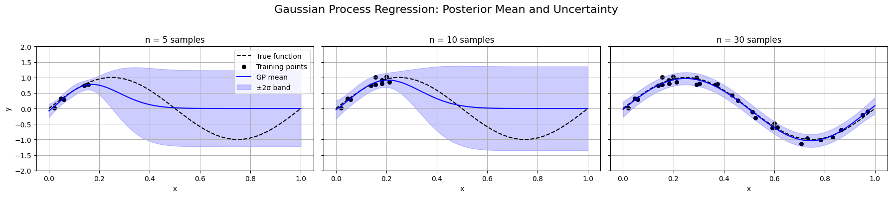
Here is a figure visualizing key concepts of Gaussian Processes with Kernel Optimization:
The GP posterior mean (blue line) adapts to increasing training data (n = 5, 10, 30).
The shaded ±2σ confidence band shows predictive uncertainty—narrowing as data increases.
The model automatically adjusts its fit through kernel hyperparameter optimization using marginal likelihood.
📌 What You Will Do in This Project#
Your clear, achievable goal is:
Implement a 1-D Gaussian Process regression model with an RBF kernel, optimizing hyperparameters via marginal likelihood maximization.
In this hands-on project, you’ll:
Code from scratch the GP predictive mean and variance calculations using a Radial Basis Function (RBF) kernel.
Implement a numerical optimization procedure (L-BFGS or simple grid search) to optimize hyperparameters:
length-scale \(\ell\),
signal variance \(\sigma_f^2\),
noise variance \(\sigma_n^2\).
Clearly visualize your fitted GP model predictions with ±2σ uncertainty bands for increasing numbers of training samples (n = 5, 10, 30).
🔍 Key Concepts You’ll Master#
Through this project, you’ll gain practical mastery of several important concepts:
Gaussian Processes fundamentals: How GP regression works as a Bayesian method, providing predictive distributions, not just single predictions.
Kernel hyperparameter optimization: Learn how to objectively tune your kernel parameters (\(\ell,\sigma_f,\sigma_n\)) by maximizing the marginal likelihood (evidence).
Numerical Stability and Efficiency: Implement the Cholesky decomposition method for stable and efficient GP inference and optimization.
Uncertainty quantification: Clearly visualize prediction uncertainty and understand its importance in real-world decision-making.
🚧 Core Tasks (Implementation Details)#
You’ll proceed with these practical steps:
RBF kernel implementation: Code up a clean and efficient RBF kernel in NumPy.
GP predictive equations: Compute the GP posterior mean and variance predictions from training data, clearly handling numerical stability (Cholesky solves and log-determinants).
Hyperparameter optimization: Use an optimizer (
scipy.optimizeor grid search) to find the best kernel hyperparameters by maximizing the marginal likelihood (evidence).Visualization of Uncertainty: Clearly plot your GP predictions with ±2σ confidence intervals for different amounts of training data (n = 5, 10, 30) to see how uncertainty evolves as more data is added.
📝 Reporting: Analysis and Insights#
Your concise report (~2 pages) should focus on clear insights, specifically:
Derivation of the GP: Derive the GP as kernelized Bayesian linear regression.
Plot how the marginal likelihood (evidence) surface changes with different values of length-scale (\(\ell\)).
Discuss over-fitting and under-fitting: What happens when your length-scale is too small or too large?
Clearly visualize how increasing data (n=5→30) reduces uncertainty and improves predictions.
🚀 Stretch Goals (Optional, Advanced)#
If you’re keen to deepen your understanding, consider:
Exploring more complex kernels (Matérn, periodic, etc.) and comparing their performance.
Implementing automatic differentiation with
scipy.optimizeor other frameworks to efficiently optimize hyperparameters.
📚 Resources and Support#
You’ll receive a starter notebook with synthetic datasets to streamline the implementation and visualization process.
Feel free to use external resources, lecture materials, and AI-assisted coding (clearly documented).
✅ Why This Matters#
Gaussian Processes are widely used in industry and research due to their powerful predictive capabilities and robust uncertainty quantification:
They are central in fields like geostatistics, finance, hyperparameter tuning, and Bayesian optimization.
Understanding GP regression deeply enhances your practical skills in probabilistic modeling and optimization—essential competencies in modern machine learning.
This project will equip you with hands-on experience, enabling you to confidently apply GPs to real-world tasks and present an insightful portfolio piece.
Project Summary: Gaussian Processes with Kernel Optimization#
(NumPy)
Item |
Details |
|---|---|
Goal |
Build 1-D GP regression with RBF kernel; learn length-scale via marginal log-likelihood maximisation (L-BFGS or grid). |
Key ideas |
Cholesky solves, log-det, automatic differentiation optional (scipy.optimize). |
Core tasks |
|
Report |
Show derivation of the GP; show how evidence surface changes with \(\ell\); comment on over/under-fitting. |
Stretch |
Explore more complex kernels (Matérn, periodic, etc.); implement automatic differentiation. |